Ridge Regression
Contents
Ridge Regression#
Ridge Regression describes an \(L_2\)-penalized regression task.
Task (Ridge Regression)
Given a dataset of \(n\) observations
the design matrix \(X\in\mathbb{R}^{n\times p}\), where \(X_{i\cdot}=\bm\phi(\vvec{x}_i)^\top\) and a regularization weight \(\lambda>0\).
Find the regression vector \(\bm\beta\), solving the following objective
Return the predictor function \(f:\mathbb{R}^d\rightarrow\mathbb{R}\), \(f(\vvec{x})=\bm\phi(\vvec{x})^\top\bm\beta\)
Optimization#
First of all, we observe that the ridge regression objective is convex. The objective function \(RSS_{L_2}\) is convex as it is the nonnegatively weighted sum of convex functions. The feasible set is the set \(\mathbb{R}^p\), which is convex as well. Hence, the whole objective is a convex, unconstrained optimization problem. That means that every stationary point of the objective function is a minimizer. We can compute the stationary points as follows:
How does this change the standard set of regression solutions?
Effect of the Regularization Weight#
The following lemma indicates that the solutions of Ridge Regression computed above are always unique (exactly one regression vector \(\beta\) solves the ridge regression objective).
Lemma 6
For any matrix \(X\in\mathbb{R}^{n\times d}\), the matrix \(X^\top X+\lambda I\) is invertible for all \(\lambda>0\)
Proof. Let \(X=U\Sigma V^\top\) be the singular value decomposition of \(X\), then
The matrix \(\Sigma^\top\Sigma +\lambda I\) is invertible, as it is a diagonal matrix where each value on the diagonal is at least as large as \(\lambda>0\). Hence, the matrix \(X^\top X+\lambda I\) is invertible and the inverse is \(V(\Sigma^\top\Sigma +\lambda I )^{-1}V^\top\).
As a result, we can multiply with \((X^\top X+\lambda I)^{-1}\) from the left in Eq. (23) and obtain the ridge regression solver.
Corollary 2
The solution to the Ridge Regression task, is given by
So, for any regularization weight \(\lambda>0\) we have a unique regression solver, but for \(\lambda=0\) we can get infinitely many solutions. Yet, what kind of solution do we get for really small \(\lambda\)? Is there one solution of the infinitely many that is somewhat better than the others? We can answer this question indeed with “yes”, as the following theorem shows.
Theorem 16
Let \(X=U\Sigma V^\top\in\mathbb{R}^{n\times p}\) be the SVD of the design matrix of the Ridge Regression task. If only \(r<p\) singular values of \(X\) are nonzero (\(X\) has a rank of \(r\)), then the global minimizer \(\bm{\beta}_{L_2}\) converges for decreasing regularization weights \(\lambda\rightarrow 0\) to
\(\Sigma_r\) denotes here the matrix containing only the first \(r\) rows and columns of the singular values matrix \(\Sigma\) and \(U_r\) denotes the matrix containing the first \(r\) left singular vectors (the first \(r\) columns of \(U\)).
Proof. We substitute \(X\) with its SVD in Eq. (23) yielding the ridge regression solutions.
We use the notation of Observation (Singular value matrix of rank r) to compute
Hence, the lower \(p-r\) rows of \((\Sigma^\top\Sigma +\lambda I )^{-1}\Sigma^\top U^\top \vvec{y}\) are equal to zero, returning
Let’s look again at the plot of Example 16. The regression function that we learn has four parameters, but we have only three data points. Hence, we have \(p-r=1\) and our regression solution vectors are computed as \(\beta=V\mathbf{w}\) where \(\vvec{w}=\begin{pmatrix}\Sigma_r^{-1} U_r^\top \vvec{y}\\ w_4\end{pmatrix}\) and \(w_4\in\mathbb{R}\). If \(w_4=0\), then the resulting \(\beta\) is the one that ridge regression converges to when \(\lambda\rightarrow 0\). We plot now the resulting regression functions, depending on the value of \(w_4\) and get the following:
import numpy as np
import matplotlib.pyplot as plt
D = np.array([5,3,1])
y = np.array([2,5,3])
def ϕ(x):
    return np.row_stack((np.ones(x.shape[0]),x, x**2, x**3))
X=ϕ(D).T
U,σs,Vt = np.linalg.svd(X, full_matrices=True)
V=Vt.T
Σ = np.column_stack((np.diag(σs),np.zeros(3)))

plt.figure(figsize=(10, 7))
x = np.linspace(0, 6, 100)

Σ_pseudoinv = Σ.copy()
Σ_pseudoinv[Σ>0] = 1/Σ[Σ>0]
w = Σ_pseudoinv.T@U.T@y
for w_4 in [0,10,20,40]:
    w[3] = w_4
    β = V@w
    f_x = ϕ(x).T@β
    plt.plot(x, f_x, label="w_4="+str(w_4))
plt.scatter(D, y, edgecolor='b', s=50)
plt.xlabel("x")
plt.ylabel("y")
plt.ylim((-5, 15))
plt.legend(loc="best")
plt.show()
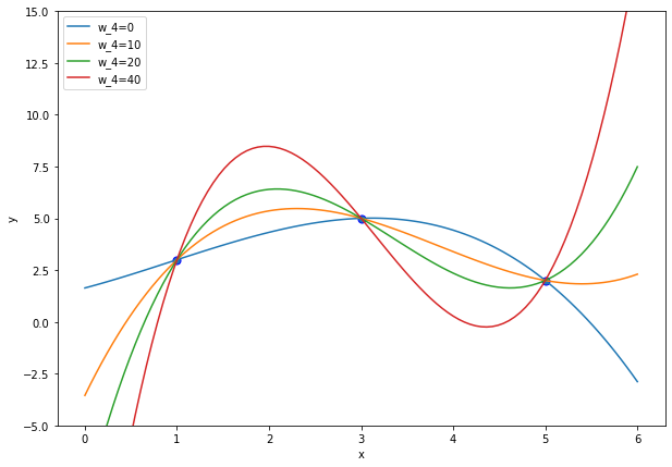
We observe that the regression function for \(w_4=0\) is not as curvy as the other ones. Generally, the higher the value of \(w_4\), the steeper are the slopes of the regression function. We can imagine that the rather erratic functions arising from high values in the parameter \(w_4\) are not desirable, as it result in a high variance among the models, depending on the training data. As a result, ridge regression gives us an idea which function we should choose when the regression objective has infinitely many solutions.
Example#
Let’s use again Example 16, but now we apply ridge regression with varying regularization weights. We implement a ridge regression solver, returning the regression parameter vector \(\beta_{L_2}\) for a given design matrix \(X\), target vector \(\vvec{y}\) and regularization weight \(\lambda\).
import numpy as np

D = np.array([5,3,1])
y = np.array([2,5,3])

def β_ridge(X, y, λ):
    p= X.shape[1]
    return np.linalg.inv(X.T@X + λ*np.eye(p))@X.T@y
Now we plot the ridge regression functions for varying regularization weights.
import matplotlib.pyplot as plt
def ϕ(x):
    return np.row_stack((np.ones(x.shape[0]),x, x**2, x**3))
X=ϕ(D).T

plt.figure(figsize=(10, 7))
x = np.linspace(0, 6, 100)
for λ in [0.001,1,10, 100]:
    β = β_ridge(X, y, λ)
    f_x = ϕ(x).T@β
    plt.plot(x, f_x, label="f_"+str(λ))
plt.scatter(D, y, edgecolor='b', s=50)
plt.xlabel("x")
plt.ylabel("y")
plt.ylim((-5, 15))
plt.axhline(0, linewidth=0.5, linestyle='--', color='gray') # horizontal lines
plt.axvline(0, linewidth=0.5, linestyle='--', color='gray') # vertical lines
plt.legend(loc="best")
plt.show()
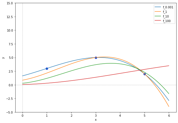
We see that the functions become with increasing penalization weight more “flat”. This is of course what we would have expected. With increasing penalization weight \(\lambda\), the minimization of the norm \(\lVert\beta\rVert^2\) becomes more important than the fit to the data expressed by the \(RSS\). But is this plot really showing you what you expected in terms of a simple function fitting to the data? After all, the idea of Ridge Regression is to regularize the learned function by putting a dampener on the coefficients of the basis functions. That is, we wanted to make the regression function more simple while still having a good fit to the data. But the regression function with high penalization weight \(\lambda=100\) is not fitting the data very well and neither does it look simple (it is curving to weirdly, basically inversely to the curvature of the data points).
Why we shouldn’t penalize the intercept#
The example shows (and it should be clear from the objective) that we obtain for a very high value of \(\lambda\) in the ridge regression objective a ridge regression vector \(\beta_{L_2}\) close to zero. That means that the resulting regression function \(f(x)=\phi(x)^\top \beta\) approximates the constant zero function when \(\lambda\rightarrow \infty\). However, whether we have an affine basis function \(f(\mathbf{x})=\beta_d x_d+\ldots \beta_1 x_1 + \beta_0\) or polynomial ones \(f(x)=\beta_2x^2+ \beta_2 x + \beta_0\), it doesn’t make much sense to penalize nonzero values of the intercept \(\beta_0\). If we penalize the intercept, then the mean of the target vector can significantly influence the resulting model. That is because a target mean that is far away from zero requires typically a higher value of the intercept to fit the regression function well to the targets. This is not desirable.
To avoid this issue, we typically exclude the intercept from regularization. In practice, this can be achieved by modifying the penalty term so that it only applies to the coefficients corresponding to the features, for example by using a diagonal matrix with a zero in the first entry (if zero is the index of the intercept):
import matplotlib.pyplot as plt

def β_ridge_intercept(X, y, λ, intercept_id):
    p= X.shape[1]
    I = np.eye(p)
    I[intercept_id,intercept_id]=0
    return np.linalg.inv(X.T@X + λ*I)@X.T@y


plt.figure(figsize=(10, 7))
x = np.linspace(0, 6, 100)
for λ in [0.001,1,10, 100, 1000]:
    β = β_ridge_intercept(X, y, λ, 0)
    f_x = ϕ(x).T@β
    plt.plot(x, f_x, label="f_"+str(λ))
plt.scatter(D, y, edgecolor='b', s=50)
plt.xlabel("x")
plt.ylabel("y")
plt.ylim((-5, 15))
plt.axhline(0, linewidth=0.5, linestyle='--', color='gray') # horizontal lines
plt.axvline(0, linewidth=0.5, linestyle='--', color='gray') # vertical lines
plt.legend(loc="best")
plt.show()
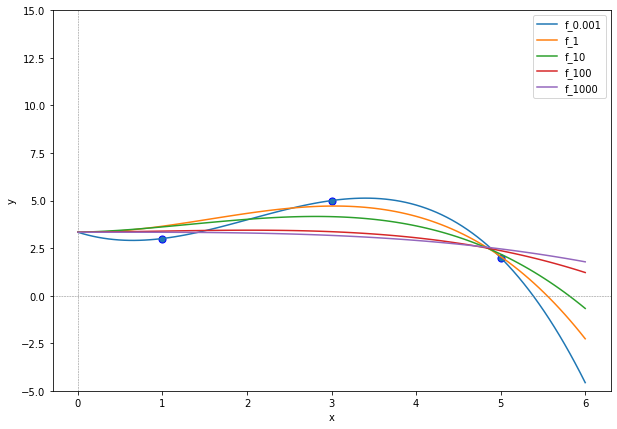
We see that the regression functions are now closer to the training data points, even for quite high penalization weights \(\lambda>100\). The regression functions also look now more simple while still fitting to the data.
We indicate the ridge regression parameters in numbers for varying regularization weights below.
for λ in [0.001,1,10, 100, 1000]:
    β = β_ridge_intercept(X, y, λ,0)
    print(λ,"\t",np.round(β,3))
0.001 	 [ 2.24   0.258  0.644 -0.141]
1 	 [ 2.504  0.22   0.55  -0.122]
10 	 [ 3.386  0.095  0.237 -0.061]
100 	 [ 3.953  0.014  0.033 -0.021]
1000 	 [ 3.978e+00  1.000e-03  2.000e-03 -1.300e-02]
We see that the resulting ridge regression parameters approximate zero for high values of \(\lambda\), but they don’t become actually zero. If we look back at the orginal motivation for applying the \(L_2\)-norm regularization, the goal to obtain sparse regression vectors and to obtain a feature selection, then we observe that ridge regression can not deliver in that use case. However, we do observe a regularizing effect in the sense that very big regularization weights get penalized by the \(L_2\)-norm regularization term.