Training
Contents
Training#
Neural networks are extremely expressive models. As suggested by the Universal Approximation Theorem, they can approximate highly complex functions if they are sufficiently big. This expressive power is their strength, but it also raises a concern about overfitting. Increasing the number of neurons in a layer or stacking more layers allows the network to learn increasingly complex functions. Yet, neural networks are often trained in a heavily overparameterized regime where classical statistical intuition would predict severe overfitting. Nevertheless, when combined with large datasets and appropriate optimization procedures, they often generalize remarkably well.
This is one of the remarkable discoveries of deep learning, that we can make the training of overcomplex models work with a combination of optimization methods, regularization techniques, and large-scale training. We discuss now the most important tricks to gain high accuracy neural network classifiers.
SGD#
Backpropagation allows us to efficiently derive the gradient of the cross-entropy loss for any network architecture. This way, we can optimize the weights of a neural network by gradient descent. However, due to the requirement of (comparably) vast amounts of data to train a neural network well, the computation of the gradient, which sums up the cross-entropy gradients for all data points, is typically too costly if the dataset is big.
Stochastic Gradient Descent (SGD) offers here a solution by updating the weights using only a small batch of training examples at a time. That is, in every update step, SGD performs a gradient descent step on the loss function
The pseudocode below indicates the procedure of SGD. For a specified number of epochs, we divide the data into batches and perform a gradient descent update on each batch.
Algorithm 11 (SGD)
Input: training data \(\mathcal{D}\), network \(f_\theta\), step-size \(\eta\)
Initialize weights \(\theta\) randomly
for epoch \(t\in\{1,\ldots,t_{max}\}\)
Divide the data into mini-batches \(\mathcal{B}_1\cup\ldots\cup\mathcal{B}_m=\mathcal{D}\)
for each batch \(\mathcal{B}\)
\(\theta\gets \theta -\eta_t\nabla \mathcal{L}(\mathcal{B},\theta)\)
Likewise, we can integrate momentum in this optimization scheme, by performing the updates with momentum on a batch only.
Properties of SGD#
SGD is not only more efficient in its computation of the gradients, it also has many theoretical advantages to gradient descent. The computation of the gradients on batches introduces noise into the gradient descent updates, that have been found to be useful in navigating complex loss landscapes and escaping local minima.
Fig. 9 gives an impression of the landscape of a neural network with only two parameters. We see how there are multiple local optima and only one very narrow valley that forms the global optimum. SGD can help in these cases, because its randomness helps to survey the loss landscape without getting stuck in smaller local minima.
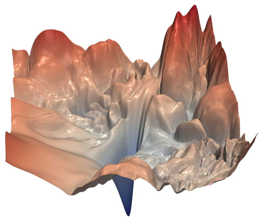
Fig. 9 Loss landscape of neural networks for a bi-dimensional parameter space (borrowed from [3]). There are several local minima and one global minimum.#
Generally, sharp minima are considered as less desirable since they are associated with poor generalization (overfitting). Flat minima often generalize better and there are some works that support that these are found with smaller batch sizes (more noisy SGD steps). Due to these properties, SGD is also considered to perform an implicit regularization. That is, although the global optimum of the loss would return a vastly overfitting model, SGD is capable to find a minimum that corresponds to a regularizing model.
However, the randomness of SGD might also be a problem when it comes to the convergence of this method. In fact, SGD requires a decreasing step-size to converge. Hence it requires a learning rate scheduler, and a good learning rate scheduler is in practice often not trivial to find. Additionally, SGD can greatly benefit from additional optimization techniques like momentum.
Training with SGD in Pytorch#
We use again the two moons dataset to demonstrate the training of a neural network. We define the function train_test that gets as input the model to optimize and a DataLoader called train_loader. The DataLoader takes care of dividing the data in batches for every epoch. We evoke the train_test function with a DataLoader of batch_size=32, meaning that each update is performed on 32 randomly sampled examples. The parameter shuffle=True reshuffles the dataset in every epoch, such that we get a new split in every epoch.
We train here a simple shallow network with a single hidden layer of 16 neurons and ReLU activation. When we perform the evaluation to track the loss and accuracy on the train and test-data, we use the command with torch.no_grad(): to perform the computations without simultaneous gradient tracking.
import torch
import torch.nn as nn
import torch.optim as optim
from torch.utils.data import DataLoader, TensorDataset
from sklearn.datasets import make_moons
from sklearn.model_selection import train_test_split
from sklearn.preprocessing import StandardScaler

# Generate and preprocess data
X, y = make_moons(n_samples=1000, noise=0.2, random_state=42)
X = StandardScaler().fit_transform(X)
X_train, X_test, y_train, y_test = train_test_split(X, y, test_size=0.2, random_state=42)

# Convert to tensors
X_train = torch.tensor(X_train, dtype=torch.float32)
y_train = torch.tensor(y_train, dtype=torch.long)
X_test = torch.tensor(X_test, dtype=torch.float32)
y_test = torch.tensor(y_test, dtype=torch.long)

# Create DataLoader for mini-batch SGD
train_dataset = TensorDataset(X_train, y_train)

def train_test(model, train_loader):
    # Define loss and optimizer
    criterion = nn.CrossEntropyLoss()
    optimizer = optim.SGD(model.parameters(), lr=0.1, momentum=0.9)

    # Store metrics
    train_accs, test_accs = [], []
    train_losses, test_losses = [], []

    # Training loop
    for epoch in range(100):
        model.train()
        for batch_X, batch_y in train_loader:
            optimizer.zero_grad()
            outputs = model(batch_X)
            loss = criterion(outputs, batch_y)
            loss.backward()
            optimizer.step()

        # Evaluate on full train/test sets
        model.eval()
        with torch.no_grad():
            train_outputs = model(X_train)
            test_outputs = model(X_test)

            train_loss = criterion(train_outputs, y_train).item()
            test_loss = criterion(test_outputs, y_test).item()
            train_losses.append(train_loss)
            test_losses.append(test_loss)

            train_preds = train_outputs.argmax(dim=1)
            test_preds = test_outputs.argmax(dim=1)

            train_acc = (train_preds == y_train).float().mean().item()
            test_acc = (test_preds == y_test).float().mean().item()

            train_accs.append(train_acc)
            test_accs.append(test_acc)

    return train_accs, test_accs, train_losses, test_losses

# Define a simple neural network model
model_sgd = nn.Sequential(
    nn.Linear(2, 16),
    nn.ReLU(),
    nn.Linear(16, 2)
)
train_loader_batch = DataLoader(train_dataset, batch_size=32, shuffle=True)
train_accs, test_accs, train_losses, test_losses = train_test(model_sgd,train_loader_batch)
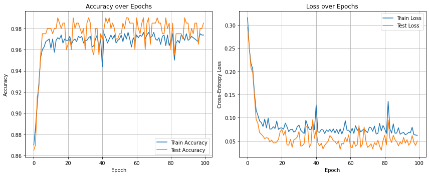
We plot the accuracy and the loss of the training and test data. Quite uncommonly, the test accuracy is here most often higher than the train accuracy. This is usually not the case and due to the low complexity of the data and a test set that probably doesn’t contain many points near the decision boundary. We observe the rather noisy progress of the trajectories.
import matplotlib.pyplot as plt

# Plot accuracy and loss side by side
fig, (ax1, ax2) = plt.subplots(1, 2, figsize=(12, 5))

# Accuracy plot
ax1.plot(train_accs, label='Train Accuracy')
ax1.plot(test_accs, label='Test Accuracy')
ax1.set_title('Accuracy over Epochs')
ax1.set_xlabel('Epoch')
ax1.set_ylabel('Accuracy')
ax1.legend()
ax1.grid(True)

# Loss plot
ax2.plot(train_losses, label='Train Loss')
ax2.plot(test_losses, label='Test Loss')
ax2.set_title('Loss over Epochs')
ax2.set_xlabel('Epoch')
ax2.set_ylabel('Cross-Entropy Loss')
ax2.legend()
ax2.grid(True)

plt.tight_layout()
plt.show()
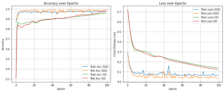
For comparison, we also train the NN architecture with gradient descent by setting the batch size equal to the size of the training set. The resulting optimization trajectories show that SGD reaches high accuracies and low losses much more quickly than gradient descent. Strictly speaking, this comparison is not entirely fair, since SGD performs multiple parameter updates within each epoch, whereas gradient descent performs only a single update. Nevertheless, the comparison remains meaningful because, after each epoch, both methods have processed the entire training dataset once.
# Define a simple neural network model
model_gd = nn.Sequential(
    nn.Linear(2, 16),
    nn.ReLU(),
    nn.Linear(16, 2)
)
train_loader_whole = DataLoader(train_dataset, batch_size=train_dataset.tensors[1].shape[0], shuffle=False)
train_accs_gd, test_accs_gd, train_losses_gd, test_losses_gd = train_test(model_gd,train_loader_whole)
# Plot accuracy and loss side by side
fig, (ax1, ax2) = plt.subplots(1, 2, figsize=(12, 5))

# Accuracy plot
ax1.plot(train_accs, label='Train Acc SGD')
ax1.plot(test_accs, label='Test Acc SGD')
ax1.plot(train_accs_gd, label='Train Acc GD')
ax1.plot(test_accs_gd, label='Test Acc GD')
ax1.set_title('Accuracy over Epochs')
ax1.set_xlabel('Epoch')
ax1.set_ylabel('Accuracy')
ax1.legend()
ax1.grid(True)

# Loss plot
ax2.plot(train_losses, label='Train Loss SGD')
ax2.plot(test_losses, label='Test Loss SGD')
ax2.plot(train_losses_gd, label='Train Loss GD')
ax2.plot(test_losses_gd, label='Test Loss GD')
ax2.set_title('Loss over Epochs')
ax2.set_xlabel('Epoch')
ax2.set_ylabel('Cross-Entropy Loss')
ax2.legend()
ax2.grid(True)

plt.tight_layout()
plt.show()
Weight Decay#
The integration of an \(L2\) regularization is integrated into Pytorch’s optimizer by the weight_decay parameter. Defining the optimizer as
optimizer = optim.SGD(model.parameters(), lr=0.1, weight_decay=0.1)
adds an \(L2\) regularization with regularization weight \(\lambda=0.1\). That is, the optimized loss is
Usually, neural network are optimized with a small value of weight decay \(\lambda \approx 0.0001\)
Dropout#
Dropout is a regularization technique that is also supposed to prevent overfitting in neural networks. During a forward pass, a dropout layer is dropping out (setting to zero) a random subset of the neurons. As a result, the network learns to perform well with a random subset of the nodes, hence reducing dependence on single nodes and being able to deal with noisy input. The resulting network is supposed to be more robust to small changes in the input. Theoretical works on the effect of dropout suggest that it results in learning weight matrices of low rank. That is, the weight matrices after a dropout layer \(W=U\Sigma V^\top\) have an SVD where only few singular values are nonzero.
The image below visualizes the effect of a dropout layer: two neurons are dropped and their input is not used in the forward pass.

The pseudocode below illustrates the operation of a dropout layer. During inference, dropout is disabled and all neuron activations are passed through unchanged. During training, however, each neuron is independently dropped with probability p. The vector \(1_u\) in Step 3 is a binary mask whose entries are equal to one for neurons that are retained and zero for neurons that are dropped. The activations of the retained neurons are passed to the next layer and scaled by a factor of \(\frac{1}{1-p}\), This scaling ensures that the expected activation remains unchanged between training and inference.
Algorithm 12 (Dropout layer)
Input: the output of the previous hidden layer \(\vvec{h}^{(\ell)}\) with dimensionality \(d_{\ell}\), the probability of dropout \(p\)
if not
trainingreturn \(\vvec{h}^{(\ell)}\)
Sample \(\vvec{u}\sim\mathcal{U}([0,1])^{d_\ell}\)
\(1_u \gets \vvec{u}>p\)
return \(\frac{1}{1-p} 1_u\circ\vvec{h}^{(\ell)} \) #element-wise product
The scaling factor may seem surprising at first. Its purpose is to compensate for the fact that, during training, only a fraction of the neurons are active. Without scaling, the total signal flowing through the network would be smaller on average during training than during inference, when all neurons are active. More formally, the scaling ensures that the expected output of a neuron is the same during training and testing.
Let \(\mathrm{dropout}(x)\) be the dropout output of hidden layer neuron \(x\), then we drop the neuron with probability \(p\) and keep it with probability \(1-p\). If we keep it, then the output is \(\frac{x}{1-p}\). Hence, the expected value of this neuron after dropout is
Thus, the expected activation remains unchanged by dropout. This allows the network to operate on approximately the same scale during both training and inference.
In Pytorch, we keep track of whether the model is trained or not by setting either model.train() or model.eval(). In evaluation mode, the dropout layer is letting through the input and the network acts deterministic. In training mode, the dropout layer is on and the model output is not deterministic. Below we define a small network with two layers, where dropout is applied in between. We sample a random input vector and compare the output of the network when training and testing. We see how the output of the model is consistent in eval mode, but not in train mode.
import torch
import torch.nn as nn

class SimpleNet(nn.Module):
    def __init__(self):
        super().__init__()
        self.fc1 = nn.Linear(10, 10)
        self.dropout = nn.Dropout(p=0.5)
        self.fc2 = nn.Linear(10, 1)

    def forward(self, x):
        x = torch.relu(self.fc1(x))
        x = self.dropout(x)
        return self.fc2(x)

model = SimpleNet()
x = torch.ones(1, 10)

with torch.no_grad():
    # During training: dropout is active
    model.train()
    y_train = model(x)
    print("Output 1 with dropout (train mode):", y_train)
    # During training: dropout is active
    y_train = model(x)
    print("Output 2 with dropout (train mode):", y_train)

    # During evaluation: dropout is disabled
    model.eval()
    y_eval = model(x)
    print("Output 1 without dropout (eval mode):", y_eval)
    # During evaluation: dropout is disabled
    y_eval = model(x)
    print("Output 2 without dropout (eval mode):", y_eval)
Output 1 with dropout (train mode): tensor([[0.5979]])
Output 2 with dropout (train mode): tensor([[0.5885]])
Output 1 without dropout (eval mode): tensor([[0.4497]])
Output 2 without dropout (eval mode): tensor([[0.4497]])