Naive Bayes
Contents
Naive Bayes#
The Naïve Bayes classifier is a simple yet powerful probabilistic algorithm used for classification tasks. It is based on Bayes’ Theorem and assumes that the features are conditionally independent, given the class label. Despite its simplicity, it performs well in many real-world applications, such as spam detection, sentiment analysis, and medical diagnosis.
Naïve Bayes is a probabilistic classifier, and before we delve into its mechanics, we establish first some terminology to describe the probabilties that we are dealing with.
Definition 31 (Probabilistic Machine Learning Speak)
Given two random variables \(\vvec{x}\) and \(y\), where \(\vvec{x}\) is the random variable of the observations of a dataset and \(y\) is the random variable of the class label. We define then the following probabilities:
\(p(y\mid \vvec{x})\) is the posterior probability (the probability of class \(y\) given observation \(\vvec{x}\) )
\(p(\vvec{x}\mid y)\) is the likelihood (how likely is it to observe \(\vvec{x}\) in class \(y\)?)
\(p(y)\) is the prior probability (how often do I expect class \(y\) to occur in my dataset?)
\(p(\vvec{x})\) is the evidence (how probable is observation \(\vvec{x}\)?)
Approximating the Bayes Classifier#
The motivation for the Naive Bayes classifier is to approximate the Bayes optimal classifier.
Goal (Naive Bayes)
Find a way to predict the most likely class
Directly estimating \(p(y\mid \vvec{x})\) is infeasible, because we would need to estimate a probability for every possible combination of feature values. That means that we would need multiple observations for each combination of feature values in order to get a reasonable estimate of the correct class probabilities. Such datasets do not exist. Imagine we have 20 binary features, then we would need more than \(2^{20}\approx 1\text{mio}\) observations to have one observation per feature combination.
Naive Bayes solves this problem by rewriting the posterior using Bayes rule and then making a naive assumption about the data that enables an efficient estimation of the required probabilities.
Theorem 19 (Bayes rule)
Given two random variables \(x\) and \(y\), then the Bayes rule is given as
The Bayes rule indicates that we can compute the unkown prediction probability \(p^*(y\mid \vvec{x})\) by means of three probabilities: the likelihood, the prior probability and the evidence. Estimating prior probabilities \(p(y)\) is easy, just return the fraction of observations with label \(y\) in the dataset. The evidence \(p(\vvec{x})\) can be neglected when we want to predict the most likely class, since it is the same for all classes:
Hence, the only thing that is left to estimate is \(p(\vvec{x}\mid y)\). This is again infeasible, because we would again need multiple observations for each feature combination and class to get a good empirical likelihood estimate. However, in contrast to the posterior probability, we can make the estimation of the likelihood feasible by making a naive assumption about the feature distribution.
Property 3 (Naive Bayes assumption)
We assume that all features are conditionally independent given the class \(y\). In this case, we can write
Under this assumption, estimating an enormous \(d\)-dimensional distribution decomposes into estimating \(d\) one-dimensional distributions. This way, we can now define the inference (prediction step) of our classifier.
Inference#
Assuming that we have computed all the probability estimations \(p(\mathtt{x}_k \mid y)\), the Naive Bayes Classifier predicts the class that is most likely, assuming class conditional independence of the features.
Definition 32 (NB classifier)
The naive Bayes classifier computes the probabilities that observation \(\vvec{x}\) occurs together with label \(y\) under the naive Bayes assumption:
As a result, the naive Bayes classifier predicts the most likely label, given observation \(\vvec{x}\):
Good applications of Naive Bayes justify the naive assumption. This assumption is for example reasonable in text classification. The features are here usually the word frequencies in a text document or the binary presence of words. Although word occurrences are generally not independent from each other, individual word occurrences can give strong independent signals to the classifier. Think of the word “viagra” when training a spam-detector. Also in medical diagnosis, Naive Bayes can be useful if the features are not strongly correlated. However, this is not always the case. For example, a prediction of a patient condition based on features like “Blood pressure”, “heart rate”, and “cholesterol levels” is not a suitable application of Naive Bayes, since these features are strongly correlated.
Implementation Practice: log probabilities#
The classifier \(f_{nb}\) multiplies \(d+1\) probabilities that have values in \([0,1]\). Especially for a high dimensional feature space (when \(d\) is large), the probabilities of \(f_{np}\) will be so close to zero that we run into numerical computation problems. Nonzero probabilities can be rounded to zero in floating-point precision. This effect is called numerical underflow. We can observe this effect in a minimal running example.
import numpy as np

# Generate 1000 random numbers in [10^{-20},1]
numbers = np.random.uniform(1e-20, 1, 1000)
product = np.prod(numbers)

print(f"Product of 1000 numbers: {product:.6e}, is the product equal to zero? {product ==0}")  # Exponential notation for clarity
Product of 1000 numbers: 0.000000e+00, is the product equal to zero? True
We can deal with underflow by computing the log-probabilities instead. After all, it doesn’t matter if we compute the prediction \(y\) that maximizes \(p(y\mid \vvec{x})\) or the \(\log p(y\mid \vvec{x})\), since the logarithm is a monotonically increasing function. As a result, we compute our classifications as
Using this log-probability trick, we get the following result for our minimal example:
z= np.sum(np.log(numbers))
z
-1040.584301739471
This way, we know that the product of the thousand numbers is equal to \(\exp(z)\), which is not equal to zero.
Multinomial Naive Bayes#
If we have discrete features \(\mathtt{x}_k\in\mathcal{X}_k\), where \(\mathcal{X}_k\) is a finite set, then we can assume multinomial probabilities \(p(\mathtt{x}_k\mid y)\) that are approximated over the counts:
Every probability \(p(\mathtt{x}_k = a\mid y=l)\) is approximated as the number of observations where feature \(\mathtt{x}_k\) is equal to value \(a\) and the label is \(y_i=l\) over the number of observations where the label is \(l\).
Implementation Practice: Laplace Smoothing#
Using the standard estimation of multinomial probabilities has the undesirable effect that some probabilities \(p(\mathtt{x}_k = a\mid y=l)\) are equal to zero if the feature \(\mathtt{x}_k\) is never equal to value \(a\) in class \(y\). In this case, the classifier probability \(f_{nb}(\vvec{x})_y\) is equal to zero for all observations \(\vvec{x}\) where \(\mathtt{x}_k=a\). In particular if we have many classes, a high-dimensional feature space or features with a large domain (if \(\mathcal{X}_k\) is large), this effect might happen quite often. Laplace smoothing mitigates this effect by adding \(\alpha\) imaginary observations for each value of \(\mathtt{x}_k\) and class \(y\).
Definition 33 (Laplace smoothing)
Given a dataset \(\mathcal{D}=\{(\vvec{x}_i,y_i)\mid 1\leq i\leq n\}\) and feature \(\mathtt{x}_k\) attaining values in the finite set \(\mathcal{X}_k\). The class-conditioned multinomial probability estimations with Laplace smoothing with variable \(\alpha> 0\) are then given as
Note that adding \(\alpha \lvert\mathcal{X}_k\rvert\) to the denominator makes the conditioned probability estimations with Laplace smoothing sum up to one:
Example 17
We consider the following toy dataset, where the task is to predict whether the email is spam, based on the words “free”, “win”, “offer” and “meeting”.
Contains “Free”? |
Contains “Win”? |
Contains “Offer”? |
Contains “Meeting”? |
Spam |
|---|---|---|---|---|
Yes |
No |
Yes |
No |
Yes |
No |
Yes |
No |
Yes |
No |
Yes |
Yes |
Yes |
No |
Yes |
No |
No |
No |
Yes |
No |
Yes |
No |
No |
Yes |
No |
No |
Yes |
Yes |
No |
Yes |
We compute the probabilities of the word “free” conditioned on whether it is in a spam email or not, using Laplace smoothing parameter \(\alpha=1\). The domain of the feature “free” is “yes” and “no”, hence, \(\lvert \mathcal{X}_{free}\rvert=2\).
Gaussian Naive Bayes#
If feature \(x_k\) attains continuous values, then a popular choice is to assume a Gaussian distribution for the class-conditioned probabilities:
The parameter \(\mu_{kl}\) is the estimated mean value \(\sigma_{kl}\) is the estimated variance of feature \(\mathtt{x}_k\) in class \(l\).
\(\mu_{kl} = \frac{1}{\lvert\{i\mid y_i=l\}\rvert}\sum_{i:y_i=l} {x_i}_k \)
\(\sigma_{kl}^2 = \frac{1}{\lvert\{i\mid y_i=l\}\rvert} \sum_{i:y_i=l} ({x_i}_k-\mu_{kl})^2\)
Note that the definition of the conditional probability for Gaussian naive Bayes is mathematically not exactly clean, since we have on the right side a probability distribution and not an actual probability. For practical purposes this is ok, since Naive Bayes relies on a comparison between likelihoods of feature values given a class.
Decision Boundaries#
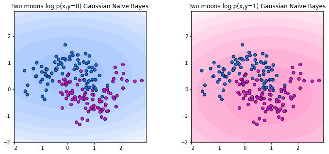
We plot the decision making process of Gaussian Naive Bayes below. The plot below shows the log probabilities of the joint distribution \(\log p(x,y)\) for each of the two classes. The more intense the color, the higher the log-probability of the corresponding class. We observe the Gaussians that are fit for each class on each axis result in an ellipse-shaped levelset.
from sklearn.naive_bayes import GaussianNB
from sklearn.model_selection import train_test_split
import matplotlib.pyplot as plt
from sklearn.inspection import DecisionBoundaryDisplay
from matplotlib.colors import ListedColormap, LinearSegmentedColormap
from sklearn.datasets import make_moons


X,y = make_moons(noise=0.3, random_state=0, n_samples=300)
X_train, X_test, y_train, y_test = train_test_split(
        X, y, test_size=0.4, random_state=42
    )

fig, axs = plt.subplots(ncols=2, figsize=(12, 5))
cm_0 = LinearSegmentedColormap.from_list("mycmap", ["#ffffff","#a0c3ff"])
cm_1 = LinearSegmentedColormap.from_list("mycmap", ["#ffffff", "#ffa1cf"])
cmaps = [cm_0,cm_1]
cm_points = ListedColormap(["#007bff", "magenta"])
for ax, k in zip(axs, (0,1)):
    gnb = GaussianNB()
    y_pred = gnb.fit(X_train, y_train)
    x = np.arange(-2, 3, 0.05)
    y = np.arange(-2, 3, 0.05)

    xx, yy = np.meshgrid(x, y)
    X = np.array([xx,yy]).reshape(2,x.shape[0]*y.shape[0]).T
    Z = gnb.predict_joint_log_proba(np.c_[xx.ravel(), yy.ravel()])
    h = ax.contourf(x,y,Z[:,k].reshape((y.shape[0],x.shape[0])),cmap=cmaps[k])

    ax.axis('scaled')
    scatter = ax.scatter(X_train[:, 0], X_train[:, 1], c=y_train, edgecolors="k",cmap = cm_points)
    _ = ax.set_title(
        f"Two moons log p(x,y={k}) Gaussian Naive Bayes"
    )

plt.show()
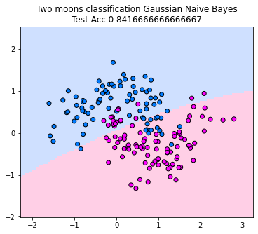
The corresponding classifier predicts the class attaining the maximum joint probability. Below, you can see the decision boundary. The classifier looks linear in this example. That is not necessarily the case, but since the joint probabilities are always ellipses, the Gaussian Naive Bayes classifier can’t model arbritary shapes in the decision boundary.
from sklearn.model_selection import train_test_split
import matplotlib.pyplot as plt
from sklearn.inspection import DecisionBoundaryDisplay
from matplotlib.colors import ListedColormap, LinearSegmentedColormap
from sklearn.datasets import make_moons


X,y = make_moons(noise=0.3, random_state=0, n_samples=300)
X_train, X_test, y_train, y_test = train_test_split(
        X, y, test_size=0.4, random_state=42
    )

_, ax = plt.subplots(ncols=1, figsize=(12, 5))
cm = ListedColormap(["#a0c3ff", "#ffa1cf"])
cm_points = ListedColormap(["#007bff", "magenta"])
gnb = GaussianNB()
y_pred = gnb.fit(X_train, y_train)
disp = DecisionBoundaryDisplay.from_estimator(
    gnb,
    X_test,
    response_method="predict",
    plot_method="pcolormesh",
    shading="auto",
    alpha=0.5,
    ax=ax,
    cmap=cm,
)
scatter = disp.ax_.scatter(X_train[:, 0], X_train[:, 1], c=y_train, edgecolors="k",cmap = cm_points)
_ = disp.ax_.set_title(
    f"Two moons classification Gaussian Naive Bayes\nTest Acc {np.mean(gnb.predict(X_test) == y_test)}"
)
ax.axis('scaled')

plt.show()
Training#
Naive Bayes doesn’t need training in the classical sense, but to enable a quick inference of a naive Bayes classifier, the required probabilities, respectively their parameters are stored in advance. That is, for discrete features we compute all log probabilities, and for continuous features we compute the estimation parameters \(\mu_{kl}\) and \(\sigma_{kl}\).
Algorithm 7 (Naive Bayes (Gaussian and Multinomial))
Input: training data \(\mathcal{D}\), \(\alpha\)
for \(k\in\{1,\ldots,d\}\)
if \(\mathtt{x}_k\) is a discrete feature
for \(a\in\mathcal{X}_k\)
for \(l\in\{1,\ldots, c\}\)
Store \(\log p_\alpha(x_k=a\mid y=l)\)
else
for \(l\in\{1,\ldots, c\}\)
Store \(\mu_{kl}\) and \(\sigma_{kl}\).