k-Means is MF

In the previous section, we introduced the k-means algorithm and saw how it minimizes an objective that captures the within-cluster scatter. But this raises several natural questions:

• How good is this algorithm?

• Does it always converge?

• Is it just a heuristic, or can we derive more general guarantees?

To answer these, we now take a step back and view k-means through the lens of the more general and powerful concept of matrix factorization. This perspective not only deepens our understanding of how k-means works, but also connects it to a broader class of unsupervised learning methods, such as truncated SVD and PCA.

Reformulating k-means as MF

At first glance, clustering and matrix factorization seem unrelated. Clustering partitions data into groups, while matrix factorization approximates a matrix with rank-one products. Surprisingly, k-means also computes a low-rank approximation of the data matrix.

Representing Cluster Assignments as a Binary Matrix

We begin by formalizing the cluster assignments using a binary indicator matrix. This indicator matrix represents simply a one-hot encoding of the vector of cluster assignments.

Example 21

Suppose we clustered four data points into two clusters, given by the following nominally encoded cluster label vector

\[\vvec{y}= \begin{pmatrix}0&1&0&1&1\end{pmatrix}\]

This indicates that points 1 and 3 belong to cluster 0, while points 2, 4 and 5 belong to cluster 1. Instead of storing the cluster labels directly, we can encode them in a binary indicator matrix:

\[\begin{split} Y= \begin{pmatrix} 1 & 0\\ 0 & 1\\ 1 & 0\\ 0 & 1\\ 0 & 1 \end{pmatrix}. \end{split}\]

Each row corresponds to one data point, and each column corresponds to one cluster. A 1 indicates membership in the corresponding cluster. A 0 indicates that the point does not belong to that cluster. Since every point belongs to exactly one cluster, every row contains exactly one entry equal to 1.

For example, the third row \((1,0)\) indicates that point 3 belongs to cluster 0, while the second row \((0,1)\) indicates that point 2 belongs to cluster 1.

Let \(Y \in \{0,1\}^{n \times r}\) be a matrix such that:

\[\begin{split} Y_{is} = \begin{cases} 1 & \text{if point } i \text{ is assigned to cluster } \mathcal{C}_s, \\ 0 & \text{otherwise.} \end{cases} \end{split}\]

Because every point belongs to exactly one cluster, every row contains exactly one nonzero entry:

\[ |Y_{i\cdot}| = 1 \quad \text{for all } i \in \{1, \dots, n\} \]

We denote by \( \mathbb{1}^{n \times r} \) the set of all such valid cluster indicator matrices:

\[ \mathbb{1}^{n \times r} = \left\{ Y \in \{0,1\}^{n \times r} \,\middle|\, |Y_{i\cdot}| = 1 \text{ for all } i \right\} \]

The Centroid Matrix

Next, we derive the matrix of cluster centroids in terms of \(Y \). We want a matrix whose columns contain the cluster centroids. Suppose we are given a data matrix \(D \in \mathbb{R}^{n \times d}\), where each row \(D_{i\cdot}\) represents a data point. The centroid of cluster \(\mathcal{C}_s\) is the mean of all points assigned to it:

\[ X_{\cdot s} = \frac{1}{|\mathcal{C}_s|} \sum_{i \in \mathcal{C}_s} D_{i\cdot}^\top = \frac{1}{|Y_{\cdot s}|} \sum_{i=1}^n Y_{is} D_{i\cdot}^\top = \frac{1}{|Y_{\cdot s}|} D^\top Y_{\cdot s} \]

We can collect all \(r\) centroids into a single matrix \(X \in \mathbb{R}^{d \times r}\), where each column \( X_{\cdot s}\) is the centroid of cluster \(s\). In matrix form, this becomes:

(68)\[\begin{split}\begin{align*} X &= D^\top Y \begin{pmatrix} \frac{1}{\lvert Y_{\cdot 1}\rvert} & &\mathbf{0}\\ &\ddots &\\ \mathbf{0}& & \frac{1}{\lvert Y_{\cdot r}\rvert} \end{pmatrix} = D^\top Y (Y^\top Y)^{-1}. \end{align*}\end{split}\]

This formula expresses the centroids as a matrix product of the data and the cluster assignments — revealing a key insight: k-means clustering can be seen as a matrix factorization problem.

The k-means objective as MF

Given a cluster assignment matrix \(Y\) and a centroid matrix \(X\), the product \(Y_{i\cdot }X^\top\) returns the centroid of the cluster to which data point \(D_{i\cdot}\) is assigned. Consequently, the matrix product \(YX^\top\) returns for every data point its assigned cluster centroid. This already suggests a connection to matrix factorization: the k-means objective in Eq. (64) minimizes the reconstruction error between the data points and their assigned centroids.

Theorem 34 (\(k\)-means MF objective)

The \(k\)- means objective in Eq. (64) is equivalent to

\[\begin{align*} \min_Y\ & RSS(X,Y) = \lVert D-YX^\top\rVert^2 &\text{s.t. }Y\in\mathbb{1}^{n\times r},\\ &&\quad X=D^\top Y (Y^\top Y)^{-1} \end{align*}\]

Proof. The matrix \(Y\) is a cluster-indicator matrix, indicating a partition of the \(n\) data points into \(r\) sets. For every data point with index \(i\in\{1,\ldots,n\}\), there exists one cluster index \(s_i\), such that \(Y_{i s_i}=1\) and \(Y_{i s}=0\) for \(s\neq s_i\) (point \(i\) is assigned to cluster \(s_i\)). Using this notation, the objective function in Eq. (64), returning the distance of every point to its cluster centroid, is equal to

\[\begin{align*} {\color{magenta}\sum_{s=1}^r}\sum_{i\in{\color{magenta}\mathcal{C}_s}}\lVert D_{i\cdot}-{\color{magenta}X_{\cdot s}^\top}\rVert^2 &= \sum_{i=1}^n{\color{magenta}\sum_{s=1}^r Y_{is}} \lVert D_{i\cdot}-{\color{magenta}X_{\cdot s}^\top}\rVert^2 &\text{(use indicator matrix)}\nonumber\\ &= \sum_{i=1}^n \lVert D_{i\cdot}-{\color{magenta}X_{\cdot {s_i}}^\top}\rVert^2&\text{(only $Y_{i s_i}=1$)}\nonumber\\ &= \sum_{i=1}^n \left\lVert D_{i\cdot}-{\color{magenta}\sum_{s=1}^rY_{is}X_{\cdot s}^\top}\right\rVert^2&\text{(only $Y_{i s_i}=1$)}\nonumber\\ &= \left\lVert D-{\color{magenta}\sum_{s=1}^rY_{\cdot s}X_{\cdot s}^\top}\right\rVert^2\label{eq:FroEuc}\\ &= \lVert D-YX^\top\rVert^2 &\text{(outer product def. matrix product)}\nonumber. \end{align*}\]

The third equation uses the composition of the squared Frobenius norm as a sum of the squared Euclidean vector norm over all rows.

The matrix factorization of k-means has a very specific structure. The left matrix \(Y\) is binary and every row contains exactly one entry being equal to one, and all the others are zero. That means, we can sort the rows of a data matrix, such that all points in one cluster have consecutive indices. The resulting matrix \(Y\) looks as the left matrix below, there is one block of ones (black) in the first column, representing the first cluster, and then follows a block of ones in the second row, representing the second cluster and so on. The right matrix \(X^\top\) indicates the centroids as the rows, each centroid has here its own color. The data matrix is then approximated over these centroids, as displayed on the right.

\(=\)

The matrix factorization of k-means, constraining the assignment matrix \(Y\) to binary values, fundamentally alters the optimization landscape of the related low-rank matrix factorization objective. In the rank-\(r\) matrix factorization problem, nonconvexity arose from the existence of many equivalent global minimizers. The nonconvexity of k-means is of a different nature. The discrete feasible set of the assignment matrix \(Y\) creates many locally optimal clustering solutions, making the optimization problem considerably more difficult.

Theorem 35

The k-means objective is nonconvex.

Proof. If we consider the penalized version of the k-means objective (putting the constraints in the main objective), then we get the following objective:

\[\begin{align*} \min_Y\ & RSS(X,Y) = \lVert D-Y (Y^\top Y)^{-1}Y^\top D\rVert^2 + \mathbb{1}_{Y\in\mathbb{1}^{n\times r}} \end{align*}\]

This objective has a local minimum for every feasible \(Y\), and inbetween the feasible points the objective returns infinity.

The discrete assignment matrix \(Y\) complicates the optimization problem, but it also provides a significant advantage, that is interpretability. In contrast to general low-rank matrix factorization, where a data point is represented as a linear combination of multiple latent factors, k-means assigns every data point to exactly one centroid. We demonstrate the interpretability of the method with our movie recommender example.

Example 22 (k-means matrix factorization for recommender systems)

Since k-means is an instance of the low-rank matrix factorization universe, we can compare the factorization of k-means in the scope of the recommender example, that we used to motivate low-rank matrix factorizations. We compute a clustering of the neutral-rating imputed running example of the recommender systems section and obtain the following:

\[\begin{align*} \begin{pmatrix} 5 & \mu & 1 & 1 \\ \mu & 1 & 5 & \mu \\\ 2 & 1 & 5 & 3 \\ 4 & \mu & 4 & 2\\ 5 & 5 & \mu & 1 \\ \mu & 1 & 5 & 3 \\ \end{pmatrix} &\approx \begin{pmatrix} 1 & 0\\ 0 & 1\\ 0 & 1\\ 1 & 0\\ 1 & 0\\ 0 & 1\\ \end{pmatrix} \begin{pmatrix} 4.7 & 3.7 & 2.7 & 1.3\\ 2.3 & 1.0 & 5.0 & 3.0\\ \end{pmatrix} \end{align*}\]

The movie patterns are now given by the centroids, and every user belongs to exactly one movie pattern, indicates by the user pattern matrix \(Y\). For example, the first user is assigned to movie pattern 1:

\[\begin{align*} \begin{pmatrix} 5 & \mu & 1 & 1 \end{pmatrix} \approx& 1\cdot \begin{pmatrix} 4.7 & 3.7 & 2.7 & 1.3 \end{pmatrix} +0\cdot \begin{pmatrix} 2.3 & 1.0 & 5.0 & 3.0 \end{pmatrix} \end{align*}\]

The k-means assignment scheme allows for a clear interpretation of the movie patterns. Each pattern indicates one user preference scheme and can hence be analyzed by itself, and not in dependence to the coefficients in \(Y\) and the other movie patterns. The example above indicates two behaviours: users that like movie one and two but not so much the other movies, and users that like movie 3.

The clustering above is obtained via sklearn:

M = [[5,3,1,1],[2,1,5,3],[2,1,5,3],[4,3,4,2],[5,5,3,1],[3,1,5,3]]
from sklearn.cluster import KMeans
kmeans = KMeans(n_clusters=2)
kmeans.fit(M)

The clustering can be obtained by kmeans.labels_ and kmeans.cluster_centers_. Sklearn labels are nominally encoded, that is, the label indicates the assigned cluster by a number. Since we have a nonconvex problem, it’s not guaranteed that you get the exact same clustering solution as above. As an exercise, you can try the code above and get the matrix factorization that is indicated by the clustering.

Convergence Analysis

The matrix factorization view provides valuable insight into the performance of Lloyds algorithm. For the matrix factorization of k-means we can show somewhat straightforwardly that fixing one of the factor matrices makes the remaining optimization problem tractable. For example, when we fix the cluster assignment matrix, then the centroid matrix is globally optimal.

Theorem 36 (Centroids as minimizers)

Given \(D\in\mathbb{R}^{n\times d}\) and \(Y\in\mathbb{1}^{n\times r}\), the minimizer of the optimization problem

(69)\[\begin{align} \min_X& \lVert D-YX^\top \rVert^2 & \text{s.t. } X\in\mathbb{R}^{d\times r} \end{align}\]

is given by the centroid matrix \(X=D^\top Y(Y^\top Y)^{-1}\).

Proof. The objective in Eq. (69) is smooth and convex. The minimizer is then given by the stationary point (FONC):

(70)\[\begin{align} \nabla_X \lVert D-YX^\top\rVert^2 = -2(D-YX^\top)^\top Y &=0\\ \Leftrightarrow D^\top Y(Y^\top Y)^{-1} &= X \end{align}\]

Likewise, when we fix the centroid matrix, then assigning each point to its closest centroid is globally optimal.

Theorem 37 (Nearest centroid assignments as minimizers)

Given \(D\in\mathbb{R}^{n\times d}\) and \(X\in\mathbb{R}^{d\times r}\), the minimizer of the optimization problem

\[\begin{align*} \min_Y& \lVert D-YX^\top \rVert^2 & \text{s.t. } Y\in\mathbb{1}^{n\times r} \end{align*}\]

is the matrix, assigning every point to the nearest centroid:

\[\begin{split}Y_{is}= \begin{cases} 1& \text{if } s=\argmin_{1\leq t\leq r}\left\{\|X_{\cdot t}-D_{i\cdot}\|^2\right\}\\ 0& \text{otherwise} \end{cases}\end{split}\]

Proof. Consider the \(k\)-means centroid objective from Eq. (64):

\[\begin{align*} \min_{\mathcal{C}_1,\ldots,\mathcal{C}_r}&\ \sum_{s=1}^r\sum_{i\in\mathcal{C}_s} \lVert D_{i\cdot}-X_{\cdot s}^\top\rVert^2\\ \text{s.t. }& X_{\cdot s}=\frac{1}{|\mathcal{C}_s|}\sum_{i\in\mathcal{C}_s}D_{i\cdot}^\top,\ \{\mathcal{C}_1,\ldots,\mathcal{C}_r\}\in\mathcal{P}_n \end{align*}\]

We replace the notation of cluster assignments via sets with the counterpart binary indicator matrix and fix the centroids. Then we have the following objective:

\[\min_{Y\in\mathbb{1}^{n\times r}}\sum_{s=1}^r\sum_{i=1}^n Y_{is}\lVert D_{i\cdot} - X_{\cdot s}^\top\rVert^2.\]

The opjective attains its minimum when we select \(Y_{is}=1 \) for the centroid with minimum distance to \(D_{i\cdot}\).

Together, Theorem 36 and Theorem 37 imply that each cluster and centroid update in Lloyds algorithm is optimal. The optimization scheme reminds of coordinate descent, only that we now do not fix all but one coordinate that we update, but we fix a block of coordinates and update the other ones in one go.

Corollary 6

Lloyds’ algorithm performs an alternating minimization (also called block coordinate descent):

\[\begin{align*} X_{k+1} & \leftarrow \argmin_{X\in\mathbb{R}^{d\times r}}\lVert D-Y_kX^\top\rVert^2\\ Y_{k+1} &\leftarrow \argmin_{Y\in \mathbb{1}^{n\times r}}\lVert D-YX_{k+1}^\top\rVert^2 \end{align*}\]

The sequence \(\{(X_k,Y_k)\}\) converges, since we decrease the objective function value in every step:

\[RSS(X_0,Y_0)>RSS(X_1,Y_1)>RSS(X_2,Y_2)>\ldots \geq 0 .\]

Because the objective is bounded below by zero, the sequence of objective values converges.

We have now encountered several formulations of the k-means problem: as within-cluster scatter minimization, as a centroid-based objective, and as a constrained matrix factorization. The following theorem summarizes that these formulations are equivalent.

Theorem 38 (Equivalent \(k\)-means objectives)

The following objectives are equivalent

(71)\[\begin{align} &\min_{Y}\ \sum_{s=1}^r\sum_{i=1}^nY_{is}\|D_{i\cdot}-X_{\cdot s}^\top\|^2 &\text{ s.t. } X\in\mathbb{R}^{d\times r}, Y\in\mathbb{1}^{n\times r}\\ &\min_{Y}\ \|D-YX^\top\|^2 &\text{ s.t. } X= D^\top Y(Y^\top Y)^{-1}, Y\in\mathbb{1}^{n\times r} \\ &\min_{Y,X}\ \|D-YX^\top\|^2 &\text{ s.t. } X\in\mathbb{R}^{d\times r},Y\in\mathbb{1}^{n\times r} \end{align}\]

Implementation

The matrix factorization view of k-means not only explains why Lloyd’s algorithm works, but also makes its implementation particularly simple. Matrix operations are efficiently implemented in Python. First, we implement some basic helper functions to get the loss and the one-hot encoded cluster assignemnt matrix.

import numpy as np
def RSS(D,X,Y):
    return np.sum((D- Y@X.T)**2)
def getY(labels):
    Y = np.zeros((len(labels), max(labels)+1))
    for i in range(0, len(labels)):
        Y[i, labels[i]] = 1
    return Y

In the following, we implement the two steps. In the centroid update, we compute \((Y^\top Y)^{-1}\) by inverting the diagonal, returning the cluster sizes (cf. Eq. (68)). If one cluster has no point assigned to it, we set the cluster size of that cluster to one, to avoid dividing by zero.
The update_assignment function computes the distances of all points to all centroids in a \(n\times r\) matrix dist. The cluster assignment is then given by the cluster with the row-wise minimum distance.
The function kmeans has as input the data matrix D, the number of clusters r, the initial centroid matrix X_init and the maximum number of iterations. The clustering and centroid updates are performed until the clustering doesn’t change anymore.

def update_centroid(D,Y):
    cluster_sizes = np.diag(Y.T@Y).copy()
    cluster_sizes[cluster_sizes==0]=1
    return D.T@Y/cluster_sizes
def update_assignment(D,X):
    dist = np.sum(D**2,1).reshape(-1,1)  - 2* D@X + np.sum(X**2,0)
    labels = np.argmin(dist,1)
    return getY(labels)
def kmeans(D,r, X_init, t_max=10000):
    rss_old,t = 0,0
    X = X_init
    Y = update_assignment(D,X)
    #Looping as long as the clustering still changes
    while rss_old != RSS(D,X,Y) and t < t_max-1:
        rss_old = RSS(D,X,Y)
        X = update_centroid(D,Y)
        Y = update_assignment(D,X)
        t+=1
        
    return X,Y

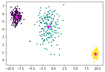
We create a synthetic dataset with 3 blob-like clusters.

from sklearn import datasets
n=500
r =3
epsilon = 0.1
D, labels = datasets.make_blobs(n_samples=n,centers=3, cluster_std=[epsilon + 0.5, epsilon + 1.25, epsilon + 0.25],random_state=7)

We run our implementation of k-means. The example is easy to cluster and k-means finds the correct clusters.

X_init = np.array([[-4,1,0.5],[0,-4,1.5]])# inital centroids
X,Y = kmeans(D,r,X_init)
import matplotlib.pyplot as plt
fig = plt.figure()
plt.scatter(D[:, 0], D[:, 1], c=np.nonzero(Y)[1], s=10)
plt.scatter(X.T[:, 0], X.T[:, 1], c='magenta', s=50, marker = 'D')
plt.show()

Initialization

The \(k\)-means problem is NP-hard, while SVD is polynomially solvable. The simple addition of binary constraints changes the complexity of the problem a lot! Although Lloyds algorithm minimizes the obective function in each step, the final result is typically a local minimum and depends strongly on the initial centroid positions.

We illustrate the sensitivity to initialization with an example. We create again a three blob dataset, but this time two of the clusters are a bit closer to each other than to the third cluster. The centroids are initialized such that they lie in the top right corner. In this example, k-means is able to distinguish the clusters perfectly.

n=500
r =3
epsilon = 0.1
D, labels = datasets.make_blobs(n_samples=n,centers=3, cluster_std=[epsilon + 0.5, epsilon + 1.25, epsilon + 0.25],random_state=1)

Once Loop Reflect

In the second example, the clusters are again initialized in the top right corner, but this time one centroid gets no points assigned and the resulting clustering is merging the two close clusters into one.

Once Loop Reflect

The simple example highlights practical challenges that arise when applying k-means. Since the objective contains many stationary clustering configurations, the quality of the final clustering can depend strongly on the initialization. As a result, practical implementations of k-means incorporate several strategies to improve robustness.

We have seen that sometimes a cluster receives no points during an assignment step. In this case, its centroid is not pulled towards the data by its assigned points, making it unlikely that the cluster will attract any points in subsequent iterations. Most implementations therefore reinitialize empty clusters, for example by placing the centroid at a randomly selected data point.

A second challenge is the choice of the initial centroids. Poor initializations may lead Lloyd’s algorithm to converge to suboptimal clustering solutions. A simple but effective strategy is to run k-means multiple times with different initializations and retain the clustering with the lowest residual sum of squares (RSS). Modern implementations often combine this idea with more sophisticated initialization schemes, such as k-means++, which aim to spread the initial centroids across the dataset and thereby reduce the likelihood of poor local optima.