Principal Component Analysis
Contents
Principal Component Analysis#
We use the Iris dataset, that we already used in the classification chapter, as a motivating example to find a low-dimensional representation of the data. You might remember that the Iris dataset indicates three classes of flowers, called versicolor, setosa, and virginica.

Fig. 11 The Iris dataset describes three Iris types#
The dataset has four features: the sepal length, width and the petal length and width.
from sklearn import datasets
import pandas as pd
iris = datasets.load_iris()
D = iris.data
y = iris.target

df = pd.DataFrame(D)
df.columns = iris.feature_names
df.head()
| sepal length (cm) | sepal width (cm) | petal length (cm) | petal width (cm) | |
|---|---|---|---|---|
| 0 | 5.1 | 3.5 | 1.4 | 0.2 |
| 1 | 4.9 | 3.0 | 1.4 | 0.2 |
| 2 | 4.7 | 3.2 | 1.3 | 0.2 |
| 3 | 4.6 | 3.1 | 1.5 | 0.2 |
| 4 | 5.0 | 3.6 | 1.4 | 0.2 |
When working with a dataset, be it for classification, regression, or unsupervised learning, it’s always a good idea to explore the data visually before jumping into modeling. This can be challenging when the dataset has many features, making direct visualization often nearly impossible. However, for datasets with a small number of features (like the Iris dataset) we can use pairwise scatter plots to gain insights. The plot below shows scatter plots for each pair of features, with points colored by class label. The diagonal displays histograms, providing an overview of the distribution of each individual feature.
from pandas.plotting import scatter_matrix
import matplotlib.pyplot as plt
import matplotlib.patches as mpatches
from matplotlib.colors import ListedColormap, LinearSegmentedColormap
import numpy as np
cm_bm = LinearSegmentedColormap.from_list("mycmapbm", ["#ffa1cf","#f37726","#a0c3ff"])
colors = np.array(["#ffa1cf", "#f37726", "#a0c3ff"])
color_array = colors[y].tolist()  # Map each row to its corresponding color


scatter_matrix(df, c =color_array, figsize=(10,10),  # c : color acording to classes
               hist_kwds={'color':'blue','bins':20, 'alpha':0.5}, alpha=1.)
# Legend
handles = [mpatches.Patch(color=colors[i], label=iris.target_names[i]) for i in range(len(iris.target_names))]
plt.legend(handles=handles, bbox_to_anchor=(1.05, 1), loc='upper left')

plt.show()
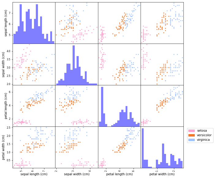
We see that some feature pairs are more suitable than others in indicating how the classes could be separated. In particular petal length vs. petal width shows that the data can possibly be linearly separated. Most views also show that the setosa class is more easy to separate from the other two classes.
Every pair of features shows us a projection of the data onto two features. The question is if we can do better than plotting pairs of features. In principle we can generate new projections or views by generating our own features. For example, we could multiply features, or compute a weighted sum of the features. The plot below shows a view of the data when plotting the sum of sepal length and width against the sum of petal length plus width.
def plot(x_1,x_2, labels=None, title="", xlabel="x", ylabel="y"):
    if labels is None:
        plt.scatter(x_1, x_2, s=25, alpha=0.5, cmap=cm_bm)
    else:
        plt.scatter(x_1, x_2, c=labels, s=25, alpha=0.5, cmap=cm_bm)
    #plt.axhline(y=0, color='m', alpha=0.5)
    #plt.axvline(x=0, color='m', alpha=0.5)
    plt.axis('equal')
    plt.xlabel(xlabel)
    plt.ylabel(ylabel)
    plt.title(title)


plot(D[:, 0]+D[:, 1], D[:,2]+D[:,3], y, title="Feature Transformation View", xlabel= iris.feature_names[0]+"+"+iris.feature_names[1], ylabel= iris.feature_names[2]+"+"+iris.feature_names[3])
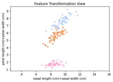
This two-dimensional view already gives a good indication on the separability of the data. The key question is if we can evaluate how good this view is, and if we could get a better low-dimensional representation of the data. To better understand what we want, we have a look at a synthetic example.
Synthetic Data Example#
Working with synthetic data is a great way to get clear about what we expect, how data is generated, and what kind of structure we are looking for in a low-dimensional view. With synthetic data we know what we put in and what we want to get out. We create a dataset that has a clear structure in 2 dimensions and then extend this data to three dimensions.
The two-dimensional dataset looks as follows:
We see that the classes, which have each their own color, are quite well separated. Now we extend this dataset to 3 dimensions by adding a third column to the dataset that is filled with Gaussian noise.
def generate3dClassData(A,labels):
    s = np.random.normal(0, 0.8, A.shape[0])
    s[labels==2] = s[labels==2]*1.4 #class 2 noise has a higher variance
    A = np.hstack([A,s[:,None]])
    return A, labels

D3d, labels = generate3dClassData(D2d,labels)
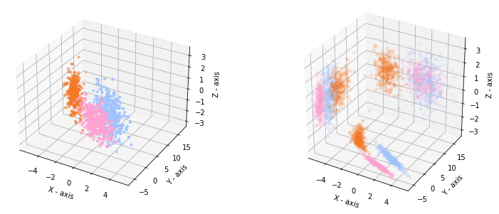
When we plot the data in a 3D plot together with the projections on each pair of features, we recognize our 2D data in the projection on the X-Y axis.
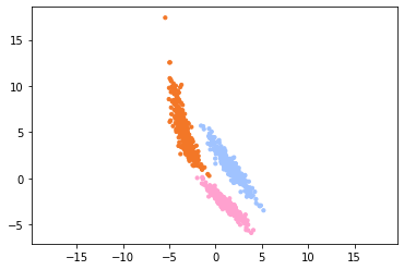
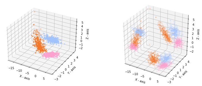
In general we cannot expect that the nicest view on the data is aligned with a selection of the axes. Hence, we rotate our 3D data to distort the two-dimensional views.
from scipy.spatial.transform import Rotation as Rt
D3d, labels = generate3dClassData(D2d,labels)
R = Rt.from_euler('zyx', [140, 145, 145], degrees=True)
D3d = D3d@R.as_matrix()
The 3D plot and the projections look now like this:
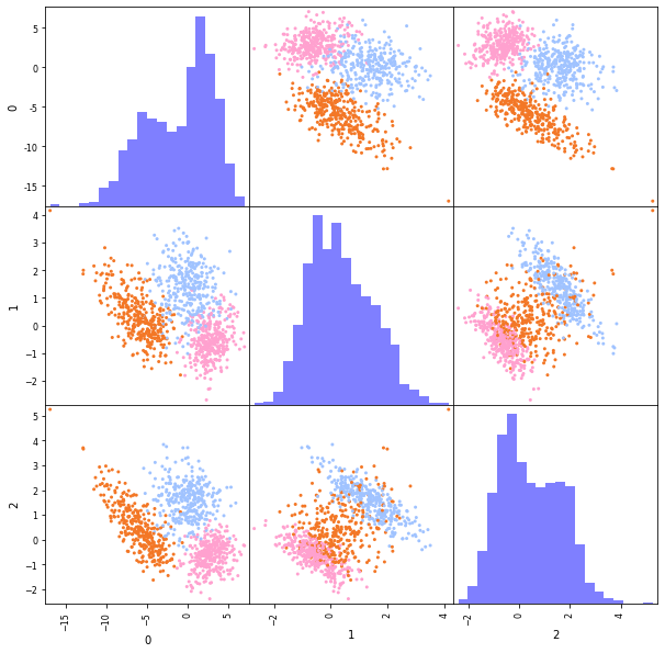
If we make a scatterplot matrix for the dataset, we get the following views. The data looks not so clearly separable anymore.
cm_bm = LinearSegmentedColormap.from_list("mycmapbm", ["#ffa1cf","#f37726","#a0c3ff"])
colors = np.array(["#ffa1cf", "#f37726", "#a0c3ff"])
color_array = colors[pd.DataFrame(labels)].squeeze()  # Map each row to its corresponding color


scatter_matrix(pd.DataFrame(D3d), c =color_array, figsize=(10,10),  # c : color acording to classes
               hist_kwds={'color':'blue','bins':20, 'alpha':0.5}, alpha=1.)
plt.show()
So, what we would like in this example is to find the direction along which we added the noise, and remove it, because this direction is not informative for the classification. Now the question is how we define the not-so informative directions. One way is to remove those directions along which not much is happening in the data. That are those directions along which the variance in the data is small.
Geometric View of PCA#
Principal Component Analysis (PCA) can be understood geometrically as a way of projecting high-dimensional data onto a lower-dimensional subspace that captures the most variation in the data. A subspace is identified by a set of vectors, that forms the basis of the subspace. Each basis vector of the subspace indicates a direction in the original feature space onto which we project the data in the low-dimensional subspace view.
Projection onto a Direction#
Mathematically, a direction can be indicated by a vector. For example, the direction onto the Z-axis in our synthetic data example is given by the vector \((0,0,1)\). From the linear algebra recap, you might remember that a projection onto a vector is given by the inner product with a unit norm vector. That means that if we want to project our data onto a direction, then we need to multiply the data points with a unit vector pointing in that direction (unit vectors have norm one).
Given the \(n\times d\) data matrix \(D\) gathering \(n\) observations of \(d\) features row-wise, the projection of all data points onto a direction indicated by vector \(\bm\alpha\) is given by
The vector \(D \frac{\bm\alpha}{\lVert\bm\alpha\rVert}\) can be interpreted as the values of a new feature, that is defined as the weighted sum of the existing features:
The newly defined feature could now represent the first feature in our low-dimensional representation. The original \(d\) features are transformed to \(r\) new features over the projections of the data onto directions.
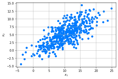
Let’s explore this by an example. We create an example dataset which has the shape of a multivariate Gaussian.
import numpy as np
mean = [10,5]
cov = [[20,10],[10,10]]
n=500

x1,x2 = np.random.multivariate_normal(mean,cov,n).T
D = np.c_[x1,x2]
dfD = pd.DataFrame(data =D,columns = ["F1","F2"])
dfD.head()
| F1 | F2 | |
|---|---|---|
| 0 | 13.710850 | 8.371449 |
| 1 | 6.304684 | 3.537377 |
| 2 | 9.492311 | 3.458008 |
| 3 | 13.504565 | 7.099266 |
| 4 | 5.625145 | -0.006308 |
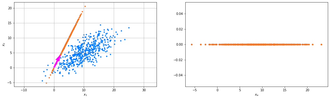
We choose vector \(\alpha=(1,2)\), creating a new feature \(\tilde{\mathtt{x}} = \frac{\alpha_1}{\lVert\bm\alpha\rVert}\mathtt{x}_1+\frac{\alpha_2}{\lVert\bm\alpha\rVert}\mathtt{x}_2\), having observations \(D\frac{\bm\alpha}{\lVert\bm\alpha\rVert}\).
α = np.array([1,2])
α=α/np.linalg.norm(α)
dfD_a = pd.DataFrame({"Da":D@α})
dfD_a.head()
| Da | |
|---|---|
| 0 | 13.619330 |
| 1 | 5.983467 |
| 2 | 7.338027 |
| 3 | 12.389202 |
| 4 | 2.509999 |
We can compute the variance in the direction of \(\bm\alpha\) as the variance of the new feature vector, that is created by projecting the data onto \(\bm\alpha\):
np.var(D@α)
19.668844927567527
Note
Pandas computes the variance in a different way than numpy does. Pandas uses the unbiased estimator (dividing by \(n-1\)) and numpy the biased estimator (dividing by \(n\)). We use the variance estimation as provided by numpy.
We plot the data (blue), the projected data (orange), and the direction onto which \(\alpha\) points (red). On the left we see how the data is projected onto the direction and on the right we see what a one-dimensional representation based on vector \(\bm\alpha\) looks like.
Variance as Information#
We have discussed what a projection of the data onto a direction looks like. But how good is the vector \(\bm\alpha\) that we chose? PCA assumes that directions with greater variance capture more information about the structure of the data. In low-dimensional projections, we want to avoid collapsing meaningful differences between data points. The example data follows a Gaussian multivariate distribution, that is defined over the variance in two directions. Of those two directions, the direction with higher variance is generally more meaningful, since this is the direction where the most happens in the data
The animation below shows the projections onto the vector indicated in red in various directions. We see that the projected data spreads more (is longer) in some directions than in others. The projections resulting in long lines are those that we’re looking for, those have a high variance.
Formal Definition of PCA#
We define the task of PCA as the task to find a basis for a low-dimensional subspace that captures the most of the variance in the data. Basis vectors have to be orthogonal and we select them in the PCA task one by one in a greedy manner, according to the variance that they capture.
Task (Principle Component Analysis)
Given a data matrix \(D\in\mathbb{R}^{n\times d}\) and a rank \(r\), denoting the number of dimensions available for.
Find the \(r\) orthogonal direction of largest variance (called principal components), given by the columns \(Z_{\cdot s}\in\mathbb{R}^d\) which are the solution to the following series of optimization problems:
Return the directions of largest variance gathered as the columns of \(Z\)
In order to understand how we can find the directions of maximum variance, we have a look how the variance \(\mathrm{var}(D\vvec{z})\) is computed for a unit vector \(\vvec{z}\).
Lemma 9
Given a data matrix \(D\in\mathbb{R}^{n\times d}\). The variance of \(D\vvec{z}\) is given as the squared norm of the centered data matrix multiplied with \(\vvec{z}\):
The vector \(\bm\mu = (\mu(D_{\cdot 1}),\ldots,\mu(D_{\cdot d}))\) is the mean vector of the data and the matrix \(C=D -\vvec{1}{\bm \mu^\top} \) is the centered data matrix (the centered data points have mean zero).
Proof. The variance is the squared deviation from the mean, and the sample mean is computed as
We compute the sample variance of the projected data as
Lemma 10
The optimization objective
is equivalent to
where \(C\) is the centered data matrix (having mean zero).
Proof. According to Lemma 9 the objective function is equal to
If we want to maximize this objective, then we can drop the scaling with \(1/n\) and we obtain the result.
The reformulation of the PCA objective according to the result above allows us to derive an optimization strategy.
Optimization#
We approach the optimization challenge of the PCA task as it is described: one principal component at a time.
Theorem 30
Let \(C\in\mathbb{R}^{n\times d}\) be a matrix, the solution of the objective
is given by the first right singular vector of \(C\). That is, if \(C=U\Sigma V^\top\) is the SVD, then the solution to the objective above is \(Z_{\cdot 1}=V_{\cdot 1}\).
Proof. If \(C=U\Sigma V^\top\) is the SVD of the centered data matrix \(C\), then we have
Since \(\sigma_1\) is the largest singular value, the objective above is maximized if \(z_1=1\) and all other coordinates being equal to zero, such that we satisfy the unit norm constraint. The solution vector \(Z_{\cdot 1}\) of the original problem is then given by \(Z_{\cdot 1}=V_{\cdot 1}\), because \(V^\top V_{\cdot 1}=(1,0,\ldots,0)\).
According to Lemma 10, the first principal component is given by the objective stated in Theorem 30. As a result, the first principal component is given by the first right singular vector of the centered data matrix.
Theorem 31
Let \(C\in\mathbb{R}^{n\times d}\) be a matrix with SVD \(C=U\Sigma V^\top\). The solution of the objective
is given by the \(s\)th right singular vector of \(C\): \(Z_{\cdot s}=V_{\cdot s}\).
Proof. We follow the same steps as in the proof of Theorem 30 and define \(\vvec{z}=V^\top Z_{\cdot s}\). Since we have \(Z_{\cdot s}^\top V_{\cdot q}=0\) for \(1\leq q < s\), the vector \(\vvec{z}\) has a specific structure:
Since \(\sigma_s\) is the largest singular value, the objective above is maximized if \(z_s=1\) and all other coordinates being equal to zero. The solution vector \(Z_{\cdot 1}\) of the original problem is then given by \(Z_{\cdot s}=V_{\cdot s}\), because \(V^\top V_{\cdot s}=(\underbrace{0,\ldots,0}_{s-1},1,0,\ldots,0)\).
As a result, the solution to PCA is given by the truncated SVD. The principal components are given by \(Z=V_{\cdot \mathcal{R}}\), where \(\mathcal{R}=\{1,\ldots,r\}\) and \(V\) is the right singular vector matrix of the centered data matrix. The principal components span the low-dimensional subspace that captures the most variance in the data. We project the data onto this subspace by multipling the data points or the centered data points with the principal components. The algorithm below details this relationship.
Algorithm 14 (PCA)
Input: \(D, r\)
\(C\gets D-\vvec{1}{\bm\mu_\mathtt{x}^\top}\) #Center the data matrix
\((U_{\cdot \mathcal{R}},\Sigma_{\mathcal{R} \mathcal{R}},V_{\cdot \mathcal{R}})\gets\)
TruncatedSVD\((C,r)\)return \(CV_{\cdot \mathcal{R}}\) #the low-dimensional view on the data
PCA can be implemented such that the low-dimensional data representation is centered (returning \(CV_{\cdot \mathcal{R}}\)) or not (returning \(DV_{\cdot \mathcal{R}}\)).
Alternative Views & Interpretations#
PCA as an Eigenvalue Problem#
The matrix \(S=C^\top C\) is the empirical covariance matrix and finding the \(s\)th-principal component can hence also be stated as the task
In this view, the principal components are given by the eigenvectors of the empirical covariance matrix \(S\). The eigenvalues indicate how much variance is captured along each direction.
PCA as Trace Optimization#
If we are not so much interested in finding the exactly ordered principal components, but more in the overall subspace that spans the low-dimensional representation of the data, we can apply the trace objective.
Theorem 32
The matrix \(Z\) that solves the objective below spans the low-dimensional subspace that is also spanned by the first \(r\) principal components.
where \(C\) is the centered data matrix.
The trace maximization objective has as global minimizers any rotation of the principal components \(Z=V_{\cdot \mathcal{R}}R\) where \(R\) is an orthogonal matrix. That has to do with the rotational invariance of the \(L_2\) matrix norm, which is induced by the trace inner product. For any solution \(Z\) and orthogonal matrix \(R\), the matrix \(ZR\) is also a solution:
PCA as a Linear Autoencoder#
PCA can be interpreted as the solution of the simplest autoencoder problem. An autoencoder is a neural network that learns a low-dimensional representation of the data by passing the input through a bottleneck and reconstructing it afterward. In general, autoencoders may contain several nonlinear layers. Here we consider a linear autoencoder, consisting of a single linear encoder and a decoder layer without activation functions.

The encoder maps the data to a \(r\)-dimensional latent representation,
where \(X\in\mathbb{R}^{d\times r}\) denotes the encoder weights. The decoder, given by the weights \(\tilde{X}\in\mathbb{R}^{d\times r}\), reconstructs the data via
The goal is to choose \(X\) and \(\tilde{X}\) such that the reconstruction error is minimized:
Let \( D = U\Sigma V^{\top}\) be the singular value decomposition of \(D\), then a global minimizer of the linear autoencoder is given by the right singular values:
That is, if the data matrix \(D\) is centered, the optimal encoding performs a projection on to the first \(r\) principal components. Note however that the factorization into \(X\) and \(\tilde{X}\) is not unique, since any rotation \(VR\) of the right singular vectors or prinscipal components with orthogonal matrix \(R\) also provides a global minimizer: