Regression Objective

Fig. 2 Example for Regression: Prediction of House Prices

Regression is a fundamental task in data mining and machine learning that aims to predict a continuous target variable from input features. A typical applications is the prediction of prices, which we explore by means of the California Housing Price Dataset. This dataset contains housing data from California districts in the 1990s and is commonly used to predict house prices based on features like median income, location, and average number of rooms. Our goal is to build a model that can accurately predict house prices based on these features. We can easily load this dataset using sklearn.

from sklearn.datasets import fetch_california_housing
california = fetch_california_housing()

print(california.DESCR)

.. _california_housing_dataset:

California Housing dataset
--------------------------

**Data Set Characteristics:**

    :Number of Instances: 20640

    :Number of Attributes: 8 numeric, predictive attributes and the target

    :Attribute Information:
        - MedInc        median income in block group
        - HouseAge      median house age in block group
        - AveRooms      average number of rooms per household
        - AveBedrms     average number of bedrooms per household
        - Population    block group population
        - AveOccup      average number of household members
        - Latitude      block group latitude
        - Longitude     block group longitude

    :Missing Attribute Values: None

This dataset was obtained from the StatLib repository.
https://www.dcc.fc.up.pt/~ltorgo/Regression/cal_housing.html

The target variable is the median house value for California districts,
expressed in hundreds of thousands of dollars ($100,000).

This dataset was derived from the 1990 U.S. census, using one row per census
block group. A block group is the smallest geographical unit for which the U.S.
Census Bureau publishes sample data (a block group typically has a population
of 600 to 3,000 people).

A household is a group of people residing within a home. Since the average
number of rooms and bedrooms in this dataset are provided per household, these
columns may take surprisingly large values for block groups with few households
and many empty houses, such as vacation resorts.

It can be downloaded/loaded using the
:func:`sklearn.datasets.fetch_california_housing` function.

.. topic:: References

    - Pace, R. Kelley and Ronald Barry, Sparse Spatial Autoregressions,
      Statistics and Probability Letters, 33 (1997) 291-297

We load the dataset as the data matrix \(D\) and the target vector \(\vvec{y}\).

D = california.data
y = california.target
n,d = D.shape

A snapshot of this dataset is given below.

import pandas as pd
df = pd.DataFrame(D,columns=california.feature_names)
df.head()

	MedInc	HouseAge	AveRooms	AveBedrms	Population	AveOccup	Latitude	Longitude
0	8.3252	41.0	6.984127	1.023810	322.0	2.555556	37.88	-122.23
1	8.3014	21.0	6.238137	0.971880	2401.0	2.109842	37.86	-122.22
2	7.2574	52.0	8.288136	1.073446	496.0	2.802260	37.85	-122.24
3	5.6431	52.0	5.817352	1.073059	558.0	2.547945	37.85	-122.25
4	3.8462	52.0	6.281853	1.081081	565.0	2.181467	37.85	-122.25

The target vector is continuous:

y

array([4.526, 3.585, 3.521, ..., 0.923, 0.847, 0.894])

The goal is to predict the target \(y\) given a feature vector \(\vvec{x}\) by means of a regression function \(f(\vvec{x})\approx y\). In our example, the function should map from an eight dimensional vector space to the real values.

We consider a subproblem first. How can we model the house price depending on the Median income feature? Below you see the plot of the first 500 data points using the feature MedInc and the target. What kind of function could describe this relationshhip?

import matplotlib.pyplot as plt
plt.figure(figsize=(10, 10))
k=0
plt.scatter(D[0:500,k], y[0:500])
plt.xlabel(california.feature_names[k])
plt.ylabel('"House prices in $100k"')
plt.show()

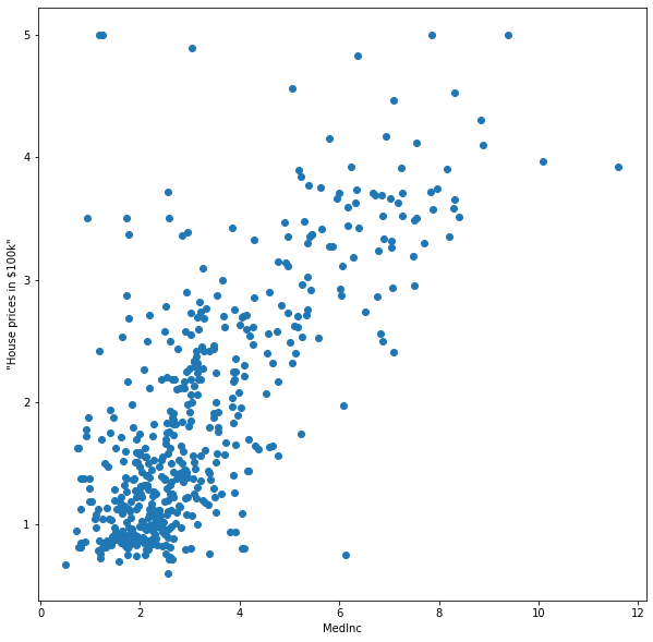
The data is scattered in a noisy cloud, but there is a visible trend. We are looking for a predictive function that captures the trend while ignoring the noise. We can formalize this idea in an informal manner.

Abstract Formalization of the Regression Task

We assume that there is some underlying function that relates the features to the price, but the observations are noisy. The underlying function is also called the true regression model function \(f^*\), generating every observation \((\vvec{x}_i,y_i)\) in the data with a random variable \(\epsilon_i\) that models the noise:

\[y_i=f^*(\vvec{x}_i)+\epsilon_i.\]

The task of regression is to approximate the underlying relationship from noisy observations. Since the true regression function is unknown, we cannot measure our error with respect to it directly. Instead, we must define our objective based only on the observed data. A natural requirement is that our predictive function should match the observed target values as closely as possible. At the same time, we restrict our search to a family of functions \(\mathcal{F}\). The choice of \(\mathcal{F}\) determines whether we allow only simple relationships or also more complex ones.

Goal (Regression)

Given a dataset consisting of \(n\) observations

\[\mathcal{D}=\left\{(\vvec{x}_i,y_i)\vert \vvec{x}_{i}\in\mathbb{R}^{d}, y_i\in\mathbb{R}, 1\leq i \leq n\right\}\]

Find a regression function \(f:\mathbb{R}^ d\rightarrow \mathbb{R}\), \(f\in\mathcal{F}\) that captures the relationship between observations and target, yielding in particular \(f(\vvec{x}_i)\approx y_i\) for all \(1\leq i \leq n\).

Measuring the Fit of a Function

To make our abstract regression task concrete, we need to define the fit of a model to the data. That is, we need to define an objective function that is small if the model \(f(\vvec{x})\) is suitable. Since our goal is to approximate the target values, we can simly measure the distance of our prediction \(f(\vvec{x})\) and the target value \(y\). The plot below indicates the distances of the predicted target (the line) to the actual data as red bars.

The distance indicated by the red bars reflect the absolute values \(\lvert y_i - f(\vvec{x}_i)\rvert\). However, the absolute value is not so easy to optimize, since it is non-differentiable at value zero. Instead, we can minimize the squared distances, which gives us a smooth objective function. Additionally, using squared distances has another side effect that might be useful: large errors are penalized more strongly, which discourages functions to deviate significantly from the data.

The squared approximation error of a function \(f\) to the target values \(y\) can be compactly written as follows for a regression function \(f(\vvec{x})\)

\[\begin{align*} RSS(\bm{\beta}) &= \sum_{i=1}^n(y_i-f(\vvec{x}_i))^2 \end{align*}\]

The function \(RSS(\bm{\beta})\) is called the Residual Sum of Squares. As the name suggests, this objective function is a sum of squared values, and is therefore convex in the residuals \(y_i-f(\vvec{x}_i)\). Now, it would be great if this objective function would also be convex in \(f\), because then we have only one globally optimal model. As you might recall from the optimization lecture, this is the case if \(f(x)\) is an affine function, because convex functions composed with affine functions remain convex. Hence, we have in the next section a look at the functions that can be expressed as a linear (hence affine) function.