Support Vector Machines

The classifiers we have seen so far have used various ways to define a decision boundary. KNN classifiers use a local view given by the neighbors, resulting in a nonlinear, typically fractured decision boundary, Naive Bayes has used elliptic (Gaussian) definitions of the likelihood to delineate between classes, and decision trees use hypercubes to define their decision boundary. Support Vector Machines (SVMs) use a hyperplane to delineate the classes, and the main motivation of the SVM is to ask what the best hyperplane is if the classes are separable. Let’s have a look at a simple example with two classes and some options for defining the separating hyperplane.

Once Loop Reflect

What do you think is the best hyperplane? Think about what happens when we want to make predictions of new data points. If a new data point is closer to the pink blob than the blue one, then we want the new point to be assigned to the pink blob. Hence, we don’t want that the hyperplane is too close to one of the blobs. The best hyperplane is the one that is equidistant to both blobs, Hyperplane 3. Mathematically, this is expressed by the idea to maximize the margin, that is twice the distance to the closest datapoint of the decision boundary. Geometrically, we want to be able to put the widest board between the classes such that all training points are left and right of the board. The plot below shows the margin boundaries for all hyperplanes.

Once Loop Reflect

We observe that Hyperplane 3 has the widest margin.

Defining Hyperplanes Mathematically

A hyperplane is a generalization of a line (in 2D) or a plane (in 3D) to any number of dimensions. In \(\mathbb{R}^d\), a hyperplane is a flat, \((d−1)\)-dimensional subspace that divides the space into two halves.

Definition 38

Given a vector \(\vvec{w}\in\mathbb{R}^d\) and value \(b\in\mathbb{R}\), then a hyperplane is defined as the set of all points satisfying the equation

\[\mathcal{H}_{\vvec{w},b} = \{\vvec{x}\in\mathbb{R}^d\mid\vvec{w}^\top \vvec{x}+b=0\}.\]

The vector \(\vvec{w}\) is called the normal vector and \(b\) is called bias.

Why are hyperplanes defined like that? We first have a look at a hyperplane with no bias (\(b=0\)). The plot below shows a hyperplane defined as \(\vvec{w}^\top \vvec{x}=0\) and the normal vector \(\vvec{w}\). Recall from Theorem 2 that a vector product with a norm one vector \(\tilde{\vvec{w}}=\vvec{w}/\lVert \vvec{w}\rVert\) has a geometric interpretation as the length of the projection of \(\vvec{x}\) onto \(\tilde{\vvec{w}}\). Hence, all vectors satisfying

\[\vvec{w}^\top\vvec{x}=0\Leftrightarrow \frac{\vvec{w}^\top}{\lVert \vvec{w}\rVert}\vvec{x}=0\Leftrightarrow \tilde{\vvec{w}}^\top\vvec{x}=0\]

land on the origin when being projected onto \(\vvec{w}\).

Now, we can define all kinds of lengths that the projection onto \(\tilde{\vvec{w}}\) shall have. For example, we can define the hyperplane that’s orthogonal to the normal vector \(\vvec{w}\) from the plot above, and that has distance two to the origin as the hyperplane

\[\frac{\vvec{w}^\top}{\lVert\vvec{w}\rVert} \vvec{x}=2\Leftrightarrow \tilde{\vvec{w}}^\top\vvec{x}=2.\]

This hyperplane is plotted below.

The hyperplane from the plot above is likewise defined as the points \(\vvec{x}\) satisfying

\[\vvec{w}^\top \vvec{x} - 2\lVert\vvec{w}\rVert=0,\]

which adheres to the general definition of a hyperplane with \(b=-2\lVert\vvec{w}\rVert\). Keep in mind, that we can interpret this hyperplane equation when dividing by the norm of the vector \(\vvec{w}\). As a result, we say that geometrically, \(\vvec{w}\) controls the slope of the hyperplane and \(b\) and \(\lVert\vvec{w}\rVert\) control the offset from the origin.

Inference of a Linear SVM for Binary Classification

A hyperplane divides a space into two halves. We assume from now on that we have only two classes, that we have a binary classification problem with labels in \(y\in\{-1,1\}\). Each hyperplane has a positive and a negative side: the positive side is the one the normal vector points to and the negative is the other side.

(38)\[\begin{eqnarray} {\bf w}^\top {\bf x} + b &<& 0\,\, \mbox{(negative side)} \nonumber \\ {\bf w}^\top {\bf x} + b &\geq& 0\,\, \mbox{(positive side)}. \nonumber \end{eqnarray}\]

Correspondingly, we can determine that the SVM predicts the positive class \(y=1\) if a point is on the positive side of the hyperplane, and the negative class otherwise. This way, we can define the inference of the SVM for the binary classification problem.

Definition 39 (SVM for binary Classification)

An SVM classifier for a binary classification problem (\(y\in\{-1,1\}\)) reflects the distance to the decision boundary \(\vvec{w}^\top \vvec{x}+b=0\). Using the sign function

\[\begin{split} \sign(a) = \begin{cases} +1 & \text{ if } a \geq 0 \\ -1 & \text{ otherwise} \end{cases}, \end{split}\]

we define the class prediction as

\[\hat{y}(\vvec{x}) = \sign(\vvec{w}^\top \vvec{x}+b).\]

Training of an SVM when Binary Classes are Separable

We assume for now that the classes are linearly separable, as in our initial example with the two blobs. That means that we can find a hyperplane (defined now as a set) \(\mathcal{H}_{\vvec{w},b}\) such that all training data points of the positive class are on the positive side, and the training data points of the negative class are on the negative side. That is, we can find \(\vvec{w}\) and \(b\) such that

\[\begin{align*} \vvec{w}^\top \vvec{x}_i+b <0 & \text{ for all } i \text{ with }y_i=-1\\ \vvec{w}^\top \vvec{x}_i+b >0 & \text{ for all } i \text{ with }y_i=1. \end{align*}\]

The equations above are satisfied if we have for all training data points

\[ (\vvec{w}^\top \vvec{x}_i+b)y_i >0. \]

The goal of the SVM is to find the hyperplane with maximum margin among all the separable hyperplanes. Hence, the SVM hyperplane maximizes the distance to the closest training data point. This way, we can define our SVM task.

Task (hard-margin SVM)

Given a binary classification training data set \(\mathcal{D}=\{(\vvec{x}_i,y_i)\mid 1\leq i\leq n, y_i\in\{-1,1\}\}\).

Find the hyperplane \(\mathcal{H}_{\vvec{w},b}=\{\vvec{x}\mid\vvec{w}^\top\vvec{x}+b=0\}\) separating the classes and having maximum margin \(2\delta\). Let \(dist(\mathcal{H}_{\vvec{w},b},\vvec{x_i})\) denote the distance of the hyperplane to training data point \(\vvec{x}_i\), then the objective of the binary hard SVM is

\[\max_{\vvec{w},b, \delta}\delta\text{ s.t. } y_i(\vvec{w}^\top\vvec{x}_i+b)\geq 0, dist(\mathcal{H}_{\vvec{w},b},\vvec{x}_i)\geq\delta \text{ for all }1\leq i\leq n\]

Return the hyperplane defining parameters \(\vvec{w},b\)

To formalize the SVM task, we need to know how we compute the distance of a point to a hyperplane. Geometrically, this works by projecting the point on the normal vector \(\vvec{w}\), giving the distance from the origin to the projection onto \(\vvec{w}\). The projection is computed by the vector product of \(\vvec{w}\) with the normed vector \(\tilde{\vvec{w}}\). From this distance, we subtract the offset from the origin \(\frac{b}{\lVert \vvec{w}\rVert}\) and we have the distance to the hyperplane. This is ilustrated in the plot below. The plot on the left shows an example where the offset to the origin is equal to two. The plot on the right annotates the distances for the more general case, where a hyperplane is defined over the formula \(\vvec{w}^\top \vvec{x}+b=0\).

As a result, we can write the distance function as

\[dist(\mathcal{H}_{\vvec{w},b},\vvec{x}_i)=\frac{\lvert\vvec{w}^\top\vvec{x}_i+b\rvert}{\lVert \vvec{w}\rVert}.\]

We observe that the constraints requiring that the classes are separated perfectly, and the ones preserving the margin are similar. In fact, we can merge these constraints. If \(y_i(\vvec{w}^\top\vvec{x}+b)\geq 0\), then we have \(y_i(\vvec{w}^\top\vvec{x}+b)=\lvert \vvec{w}^\top\vvec{x}+b\rvert\), and hence we can write

\[dist(\mathcal{H}_{\vvec{w},b},\vvec{x}_i)=\frac{y_i(\vvec{w}^\top\vvec{x}_i+b)}{\lVert \vvec{w}\rVert}.\]

This allows us to simplify the Hard Margin SVM task, by replacing the two constraints by one:

\[\begin{align*} \max_{\vvec{w},b,\delta}\delta \text{ s.t. } \frac{y_i(\vvec{w}^\top\vvec{x}_i+b)}{\lVert \vvec{w}\rVert}\geq \delta. \end{align*}\]

This objective looks already much better, but we can simplify it even more. We rewrite the constraint by multiplying with the norm of \(\vvec{w}\)

\[ y_i(\vvec{w}^\top\vvec{x}_i+b)\geq \delta \lVert \vvec{w}\rVert. \]

For any given \(\delta\) we can scale \(\vvec{w}\) such that \(\delta \lVert \vvec{w}\rVert=1\). In this case, the minimum distance of a data point to the hyperplane is \(\delta = \frac{1}{\lVert\vvec{w}\rVert}\). We substitute this into our objective and get

\[\begin{align*} \max_{\vvec{w},b}\frac{1}{\lVert\vvec{w}\rVert} \quad\text{ s.t. } y_i(\vvec{w}^\top\vvec{x}_i+b)\geq 1. \end{align*}\]

This objective is already pretty good but the maximum of \(\frac{1}{\lVert\vvec{w}\rVert}\) is reached when \(\lVert\vvec{w}\rVert\rightarrow 0\). This can result in numerical instabilities, since we don’t want to divide by zero. This issue is easily solved by minimizing \(\lVert\vvec{w}\rVert^2\) instead. We use the squared norm because this is easier to optimize than applying the square root from the Euclidean norm. As a result, we can conclude the following theorem, specifying the hard margin SVM objective.

Theorem 20 (Hard Margin SVM objective)

The following objective solves the Hard Margin SVM task

\[\min_{\vvec{w},b}\lVert \vvec{w}\rVert^2\text{ s.t. } y_i(\vvec{w}^\top\vvec{x}_i+b)\geq 1 \text{ for all }1\leq i\leq n.\]

The plot below provides a geometric interpretation of the hard margin SVM objective:

• The minimum distance of a training data point to the hyperplane is given as \(\frac{1}{\lVert\vvec{w}\rVert}\).

• The training data points that are at minimum distance to the hyperplane are called support vectors.

• The SVM decision boundary defined over the equation \(\mathbf{w}^\top \mathbf{x} +b = 0\).

• The hyperplanes that go through the support vectors are defined over the equation \(\mathbf{w}^\top \mathbf{x} +b = \pm 1\).

• The margin is defined as \(\frac{2}{\lVert\vvec{w}\rVert}\), can be interpreted as the width of the thickest board that can be put inbetween the classes.

Optimization

The SVM objective is constrained. Hence, a natural choice to solve the objective is to formulate the dual. We formulate our primal objective such that the constraints are of the form \(g_i(\vvec{x})\geq 0\):

\[\min_{\vvec{w},b}\ \lVert \vvec{w}\rVert^2\quad\text{ s.t. } y_i(\vvec{w}^\top\vvec{x}_i+b)-1\geq 0 \text{ for all }1\leq i\leq n.\]

We can now specify the Lagrangian:

(39)\[\begin{align*} \mathcal{L}((\vvec{w},b),\bm\lambda) = \lVert \vvec{w}\rVert^2 - \sum_{i=1}^n \lambda_i(y_i(\vvec{w}^\top\vvec{x}_i+b)-1) \end{align*}\]

The Lagrangian is convex with respect to \(\vvec{w}\) and \(b\), it is the sum of the convex squared L2 norm and affine functions. Hence, the stationary points subject to \(\vvec{w}\) and \(b\) are the minimizers of the Lagrangian. Hence, we write

(40)\[\begin{split}\begin{align*} \nabla_{\bf w} {\cal L}((\vvec{w},b), \bm\lambda) &= 0 \Leftrightarrow {\bf w} = \frac12\sum_{i=1}^{n} \lambda_{i} y_i {\bf x}_i\\ \frac{\partial {\cal L}((\vvec{w},b), \bm\lambda)}{\partial b} &= 0 \Leftrightarrow \sum_{i=1}^{n} \lambda_i y_i = 0. \end{align*}\end{split}\]

Now, we plug in the results from above to obtain the dual objective function:

\[\begin{align*} {\cal L}_{dual}(\bm\lambda) &=\left\lVert \frac12\sum_{i=1}^{n} \lambda_{i} y_{i} {\bf x}_{i}\right\rVert^2 - \sum_{i=1}^n \lambda_i\left(y_i\left(\frac12\sum_{j=1}^{n} \lambda_{j} y_{j}\vvec{x}_j^\top\vvec{x}_i+b\right)-1\right)\\ &=\frac{1}{4} \sum_{i=1}^{n} \sum_{j=1}^{n} \lambda_{i} \lambda_{j} y_{i} y_{j} {\bf x}_{i}^\top {\bf x}_{j} - \frac12\sum_{i=1}^{n} \lambda_{i}y_{i} \sum_{j=1}^{n} \lambda_{j} y_{j} {\bf x}_{j}^\top {\bf x}_{i} - \underbrace{\sum_{i=1}^{n} \lambda_{i} y_{i}}_{= 0} b + \sum_{i=1}^{n} \lambda_{i} \\ &= - \frac{1}{4} \sum_{i=1}^{n} \sum_{j=1}^{n} \lambda_{i} \lambda_{j} y_{i} y_{j} {\bf x}_{i}^\top {\bf x}_{j} + \sum_{i=1}^{n} \lambda_{i}. \end{align*}\]

As a result, our dual objective looks now as follows:

Theorem 21 (Hard Margin Dual)

The dual optimization objective to the Hard Margin SVM task is given as

(41)\[\begin{split}\begin{align*} \min_{\boldsymbol{\lambda}} & \frac{1}{4} \sum_{i=1}^{n} \sum_{j=1}^{n} \lambda_{i} \lambda_{j} y_{i} y_{j} {\bf x}_{i}^\top {\bf x}_{j} - \sum_{i=1}^{n} \lambda_{i} \\ \text{s.t. } & \sum_{i=1}^{n} \lambda_{i} y_{i} = 0,\ \lambda_{i}\geq 0, \text{ for all } 1\leq i\leq n. \end{align*}\end{split}\]

The dual objective is a convex optimization problem. In particular, it is a so-called quadratic program for which many solvers exist.

Theorem 22 (Quadratic Program Hard Margin)

The dual optimization objective to the Hard Margin SVM task is equivalent to the following convex quadratic program

(42)\[\begin{split}\begin{align*} \min_{\boldsymbol{\lambda}}\ & \bm{\lambda}^\top Q\bm{\lambda} - \bm{\lambda}^\top\mathbf{1} \\ \text{s.t. } & \bm{\lambda}^\top \vvec{y} = 0,\ \lambda_{i}\geq 0, \text{ for all } 1\leq i\leq n, \end{align*}\end{split}\]

where \(Q=\frac14 \diag(\vvec{y})DD^\top\diag(\vvec{y})\in\mathbb{R}^{n\times n}\) is defined over the data matrix \(D\in\mathbb{R}^{n\times d}\), gathering all data points over its rows \(D_{i\cdot}=\vvec{x}_i\) and \(\mathbf{1}\in\{1\}^n\) is the constant one vector.

Proof. We show that the objective above is convex.

• The objective function is convex: the function

\[\begin{align*}\vvec{x}^\top Q\vvec{x} = \vvec{x}^\top \frac14 \diag(\vvec{y})DD^\top\diag(\vvec{y})\vvec{x} = \frac14\lVert D^\top\diag(\vvec{y})\vvec{x}\rVert^2 \end{align*}\]

is convex because it is a composition of a convex function (the squared L2 norm) and an affine function. Hence the objective function of the quadratic program is the sum of a convex function \(\bm{\lambda}^\top Q\bm{\lambda}\) and a linear function \(-\bm{\lambda}^\top\mathbf{1}\) and hence convex.

• The feasible set is convex: the feasible set is the nonnegative subspace of a hyperplane, defined by \(\bm{\lambda}^\top\vvec{y}=0\) and is hence a convex set. As a result, the objective above is convex.

Once we have solved the convex program, we can obtain the optimal hyperplane from the Lagrange multipliers. This is necessary to perform the inference step, the classification for unseen data points.

Theorem 23 (Optimal hyperplane)

Given the minimizer \( \boldsymbol{\lambda}^{\ast} \) of (42), the solution to the Hard Margin SVM task is given by

(43)\[\begin{split}\begin{align*} {\bf w}^{\ast} &= \sum_{i=1}^{n} \lambda_{i}^{\ast} y_{i} {\bf x}_{i}\\ b^{\ast} &= y_{i} - {{\bf w}^{\ast}}^\top {\bf x}_{i} \quad\text{ for any }i\text{ such that } \lambda_{i} > 0 , \end{align*}\end{split}\]

Proof. According to Slater’s condition, we have strong duality for the SVM objective and hence, solving the dual gives also the solution to the primal problem. The definition of minimizer \(\vvec{w}^*\) follows from Eq.(40) and the optimal bias term is computed based on the fact that some data points have to lie exactly on the margin hyperplanes, because otherwise, we could increase the margin until we touch points with the margin hyperplanes.

\[\begin{align*} y_i(\vvec{w}^\top\vvec{x}_i+b)=1\ & \Leftrightarrow b=\frac{1}{y_i}-\vvec{w}^\top\vvec{x}_i\\ &\Leftrightarrow b=y_i-\vvec{w}^\top\vvec{x}_i. \end{align*}\]

The last equality follows from the fact that \(y_i\in\{-1,+1\}\).
We can indentify the support vectors as those vectors \(\vvec{x}_i\) for which \(\lambda_i>0\). There needs to be at least one \(\lambda_i>0\), because otherwise the Lagrangian in Eq.(39) would be equal to \(\lVert\vvec{w}\rVert^2\) and the margin could be maximized further, hence we wouldn’t be at the global minimum.

Training of an SVM when Binary Classes are Non-Separable

The case where we have linearly separable classes is good to formulate the idea of the optimal hyperplane, but in practice we will most likely not encounter a linearly separable classification dataset. Real-world data is often noisy or overlapping, making perfect separation impossible. To handle this, we extend the SVM formulation to allow some misclassifications by introducing slack variables, which measure the degree of violation of the margin constraints.

These slack variables, denoted by \(\xi_i\geq 0\), allow individual data points to be on the wrong side of the margin — or even the hyperplane — by “paying a penalty” in the objective function. The modified optimization problem aims to balance maximizing the margin with minimizing the total slack, effectively trading off model complexity with training error. This leads to what is known as the soft-margin SVM, which is more robust and practical for real-world classification tasks. In the plot below, we indicate how these penalties can work. We have one blue and one red point that reach into the margin area. The blue point is still on the right side of the decision boundary, it satisfies the equation \(\vvec{w}^\top\vvec{x}+b = 1-\xi> 0\), hence \(\xi_i<1\). The red point crosses the decision boundary, it satisfies the equation \(\vvec{w}^\top\vvec{x}+b = -1+\xi> 0\), hence \(\xi>1\).

We formulate the task of the soft-margin SVM below. The objective function includes now the penalty term \(\sum_{i=1}^n\xi_i\) with regularization weight \(C\). The larger \(C\) is, the more are violations of the margin boundaries penalized.

Task (soft-margin SVM)

Given a binary classification training data set \(\mathcal{D}=\{(\vvec{x}_i,y_i)\mid 1\leq i\leq n, y_i\in\{-1,1\}\}\) and parameter \(C>0\).

Find the hyperplane defined as all points in the set \(\{\vvec{x}\mid\vvec{w}^\top\vvec{x}+b=0\}\) separating the classes and having maximum margin.

\[\min_{\vvec{w},b,\bm\xi}\lVert \vvec{w}\rVert^2+C\sum_{i=1}^n\xi_i\quad\text{ s.t. } y_i(\vvec{w}^\top\vvec{x}_i+b)\geq 1 -\xi_i,\ \xi_i\geq 0 \text{ for }1\leq i\leq n\]

Return the hyperplane defining parameters \(\vvec{w},b\)

Optimization

The optimization of the soft-margin SVM is similar to the hard-margin SVM. We define the dual objective and apply a quadratic solver.

Theorem 24

The dual optimization objective to the Soft-Margin SVM task is given as

(44)\[\begin{split}\begin{align*} \max_{\boldsymbol{\lambda}} & - \frac{1}{4} \sum_{i=1}^{n} \sum_{j=1}^{n} \lambda_{i} \lambda_{j} y_{i} y_{j} {\bf x}_{i}^\top {\bf x}_{j} + \sum_{i=1}^{n} \lambda_{i} \\ \text{s.t. } & \sum_{i=1}^{n} \lambda_{i} y_{i} = 0 \\ & 0 \leq \lambda_{i} \leq C, \quad \text{ for }1\leq i\leq n. \end{align*}\end{split}\]

Proof. The Lagrangian is given as

\[\begin{align*} \mathcal{L}((\vvec{w},b,\bm{\xi}),\bm{\lambda},\bm{\mu}) = \lVert\vvec{w}\rVert^2 +C\sum_{i=1}^n\xi_i -\sum_{i=1}^n\lambda_i(y_i(\vvec{w}^\top\vvec{x}_i +b)-1+\xi_i) -\sum_{i=1}^n\mu_i\xi_i, \end{align*}\]

where \(\lambda_i,\mu_i\geq 0\) are Lagrange multipliers. Setting the gradients subject to the parameters to zero yields

\[\begin{align*} \nabla_{\bf w} {\cal L}((\vvec{w},b,\bm{\xi}),\bm{\lambda},\bm{\mu}) &= 0 \Leftrightarrow {\bf w} = \frac12\sum_{i=1}^{n} \lambda_{i} y_{i} {\bf x}_{i}\\ \frac{\partial {\cal L}((\vvec{w},b,\bm{\xi}),\bm{\lambda},\bm{\mu})}{\partial b} &= 0 \Leftrightarrow \sum_{i=1}^{n} \lambda_{i} y_{i} = 0\\ \frac{\partial {\cal L}((\vvec{w},b,\bm{\xi}),\bm{\lambda},\bm{\mu})}{\partial \xi_i} &= 0 \Leftrightarrow C = \lambda_i + \mu_i. \end{align*}\]

Plugging in those results yields the dual objective function that is stated above. The Lagrange multipliers \(\mu_i\) are not needed, since we can replace the condition \(\mu_i\geq 0\) with \(\lambda_i\leq C\), since \(\lambda_i=C-\mu_i\).

Likewise, we formulate the quadratic program of the soft-margin SVM.

Corollary 3 (Quadratic Program Soft-Margin)

The dual optimization objective of the Soft-Margin SVM task is equivalent to the following convex quadratic program

(45)\[\begin{split}\begin{align*} \min_{\boldsymbol{\lambda}} \ & \bm{\lambda}^\top Q \boldsymbol{\lambda} + {\bf 1}^\top \boldsymbol{\lambda} \\ \text{s.t. } & \boldsymbol{\lambda}^\top{\bf y} = 0 \\ & 0 \leq \lambda_{i} \leq C, \text{ for }1\leq i\leq n, \end{align*}\end{split}\]

where \(Q=\frac14 \diag(\vvec{y})DD^\top\diag(\vvec{y})\in\mathbb{R}^{n\times n}\) is defined over the data matrix \(D\in\mathbb{R}^{n\times d}\), gathering all data points over its rows \(D_{i\cdot}=\vvec{x}_i\) and \(\mathbf{1}\in\{1\}^n\) is the constant one vector.

Example 18

The plot below shows the effect of the results of the soft SVM with varying regularization weights \(C\). We state the decision boundaries for \(C\in\{0.1,1,100\}\). Using large weights such as \(C=100\) is common for the SVM. The larger \(C\) is, the more does the decision boundary adapt to the points that are closest to it, which are the first to introduce a penalty on margin or decision boundary violations.

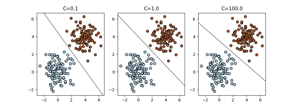
Fig. 4 Linearly separable dataset.

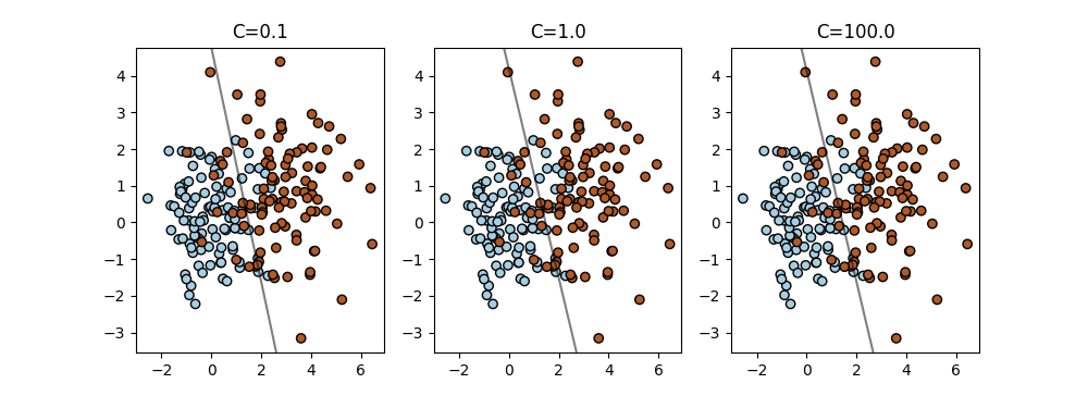
Fig. 5 Linearly non-separable dataset.