Matrix Decompositions: Why and How
When we want to talk about matrix factorizations, then we have to start at the beginning: the eigendecomposition and the singular value decomposition. There are so many aspects about these decompositions, I don’t think that we will have time to explore them. Here, I just want to talk about the somewhat less known but nevertheless imposrtant optimization problems which these decompositions solve. Let’s just take what we need from the vast theory about these decompositions and run with it.
Singular Value Decomposition
Any real-valued matrix has a Singular Value Decomposition (SVD). SVD provides a very efficient representation of a matrix and shows its characteristics. Yet, SVD is not just SVD: there are multiple representations and each has its own merits. Let us start with the full representation, sketched in the following picture.
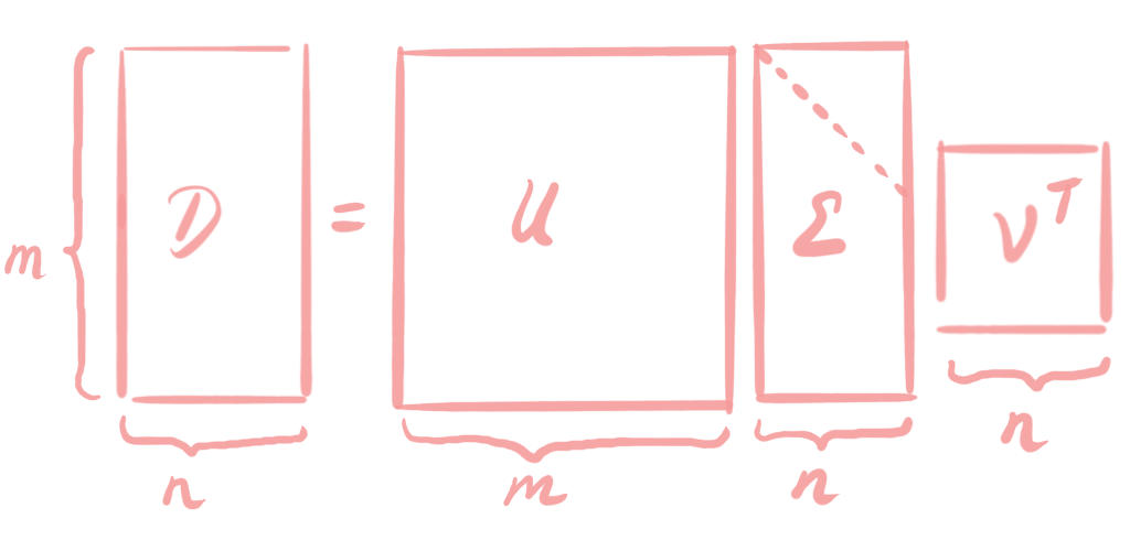 The $m\times n$ matrix $D$ is decomposed into three matrices $U,V$ and $\Sigma$. $U$ and $V$ are orthogonal matrices, it holds that
where $I_m$ and $I_n$ are the $m$- and $n$-dimensional identity matrices. The good thing about orhogonal matrices is that they are invertible, and that we can easily compute the inverse by transposing the matrix. This allows us to play with the elements of SVD. We can bring the orthogonal matrices from one side of the equation to the other side, by multiplying with the inverse. Hence, if we multiply with $V$ from the right, we get:
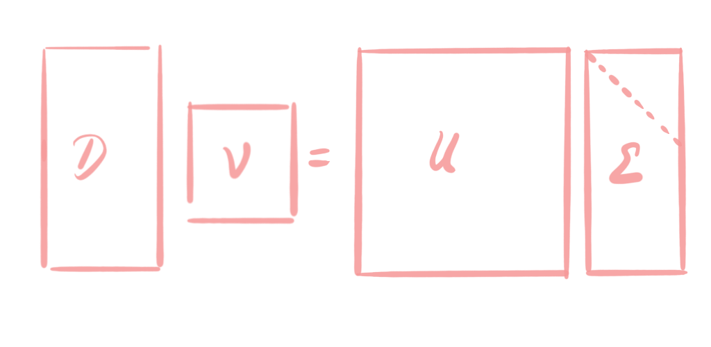 Now, if we multiply with $U^\top$ from the left, we get
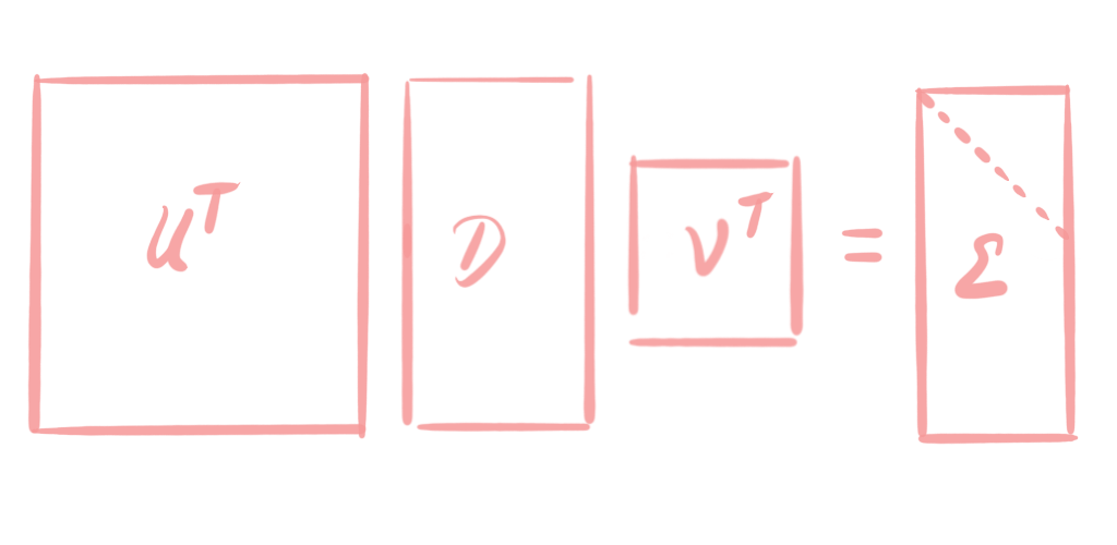 This way, we transform our matrix $D$ into a block-diagonal matrix. $\Sigma$ is a block-diagonal matrix, which has the singular values $\sigma_1\geq\ldots\geq \sigma_n\geq 0$ on its diagonal. Singular values are always nonnegative, hence $\Sigma$ is nonnegative. If $m\neq n$, like in our example, then $\Sigma$ is composed by a diagonal matrix (the upper part) and a zero matrix (the lower part). We can separate the diagonal part of $\Sigma$ from the zero part by the matrix multiplication rules. When multiplying $U$ with $\Sigma$, the blue part of $U$ is multiplied with the blue part of $\Sigma$, as visualized in the following picture:
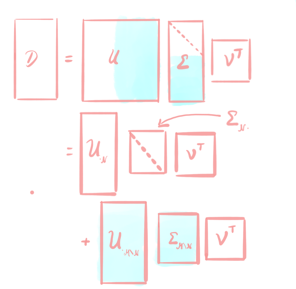 .
So, here we denote the column indices with the sets $\mathcal{N}={1,\ldots,n}$ and $\mathcal{M}={1,\ldots,m}$. The matrix $\Sigma_{\mathcal{M}\setminus\mathcal{N}\cdot}$ denotes the lower, blue part of $\Sigma$, which is entirely filled with zeros. Hence, the second term of the sum is a zero matrix and can be omitted from the sum. This leaves us with the following, shorter representation of SVD:
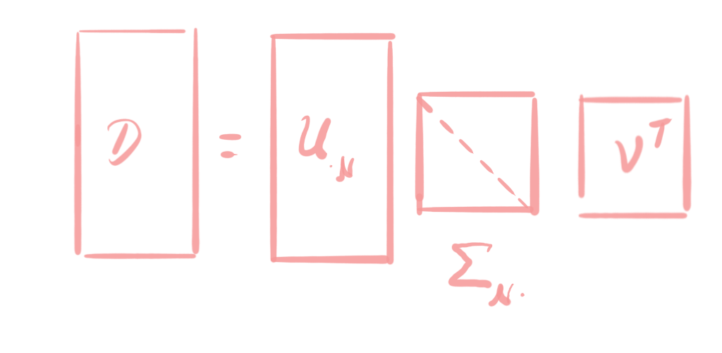 Here, we have now a diagonal middle matrix, but the left matrix $U_{\cdot\mathcal{N}}$ is not orthogonal anymore if $n<m$. If $n<m$, we have $U_{\cdot\mathcal{N}}^\top U_{\cdot\mathcal{N}} \neq U_{\cdot\mathcal{N}} U_{\cdot\mathcal{N}}^\top $ because the one is an $n\times n$ matrix and other is an $m\times m$ matrix. $U_{\cdot\mathcal{N}}$ does still have orthogonal columns, though. That is, we still have $U_{\cdot\mathcal{N}}^\top U_{\cdot\mathcal{N}}=I_n$.
Now, let’s have another look at the middle diagonal matrix. Now, if one or more singular values $\sigma_k=\ldots=\sigma_n=0$ are equal to zero, then we have again the case that the middle matrix is composed of a diagonal part and a zero part. The zero part is again visualized in blue here, and by applying the same trick as above, we can again omit the blue part from the matrix multiplication. Therewith, we get an even shorter representation of SVD:
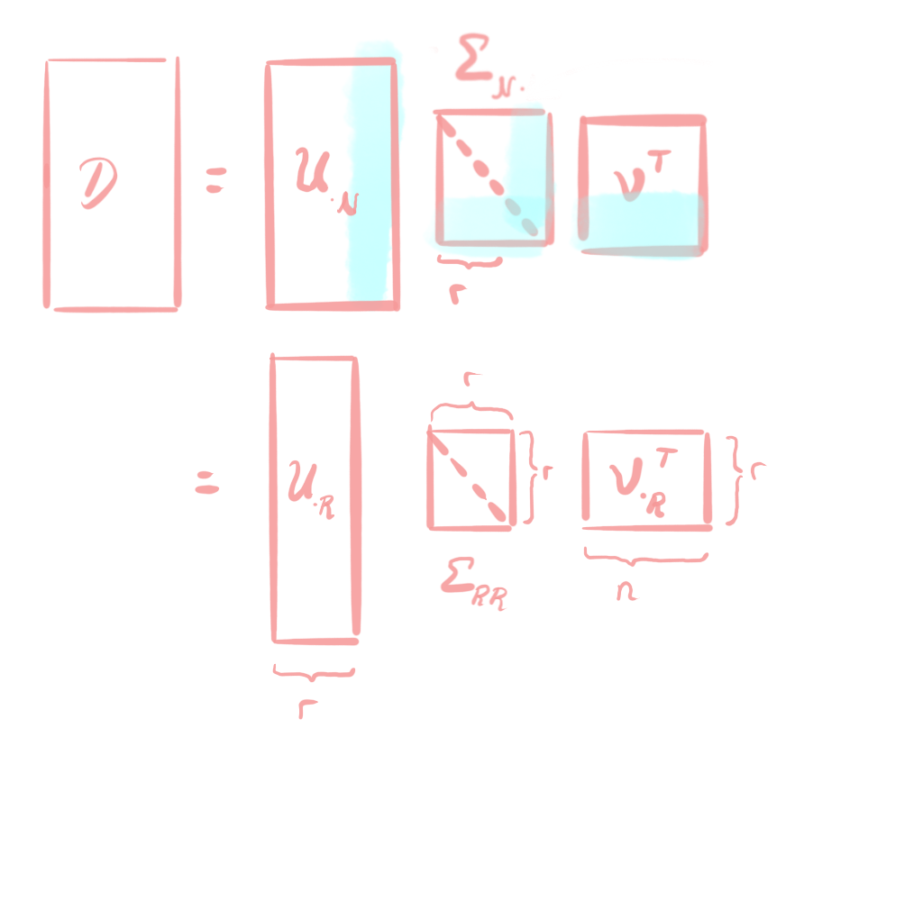 The number $r$ of the nonzero singular values is the rank of the matrix $D$.
What to do with SVD?
Ok cool, we have now this SVD of a matrix. But why?
